|
|
|
|
Fast time-to-depth conversion and interval velocity estimation in the case of weak lateral variations |
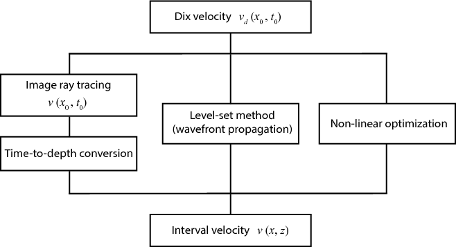
Conventional time-to-depth conversion involves an application of Dix inversion, which is strictly valid only in laterally homogeneous models. The effects from lateral velocity variations can cause unstable inversion and produce inaccurate results (Lynn and Claerbout, 1982; Black and Brzostowski, 1994; Blias, 2009; Bevc et al., 1995; Sripanich et al., 2017). Cameron et al. (2007) and Cameron et al. (2008) showed that converting seismic images from the distorted time coordinates to the Cartesian depth coordinates in the presence of lateral velocity variations amounts to solving an inverse problem specified by a system of partial differential equations (PDEs) that describes the kinematics and geometrical spreading of image rays (Hubral, 1977). Solving this system involves finding an accurate interval velocity and coordinates maps from the time domain to the depth domain. Figure 1 shows a schematic of two general paths adopted in previous works. The first approach begins with the estimation of interval velocity still expressed in the time domain from image ray tracing followed by a time-to-depth conversion using a Dijkstra-like solver (Cameron et al., 2007,2008,2009). The second approach combines the two steps together and proceeds by propagating an image wavefront (Valente et al., 2017; Cameron et al., 2007). An extension of the problem along 2D profiles to 3D was discussed by Iversen and Tygel (2008). For the third approach, Li and Fomel (2015) proposed to formulate this inversion in a non-linear iterative optimization framework supplied with regularization for better handling of its ill-posedness. This method allows for a global update of the estimated interval velocity at each iteration, which is generally preferable to solutions from time-stepping along the image rays in other known methods.
|
|---|
|
t2dnew
Figure 1. A schematic illustrating the general approaches to time-to-depth conversion and interval velocity estimation. |
|
|
In this paper, we consider the case of mild lateral variations and propose to approximate the original system of PDEs to limit our consideration to their first-order perturbative effects. This linearization leads to a notable simplification and a higher efficiency, while still correcting the conventional Dix inversion for lateral variations. The result from this approach can be used as an initial velocity model for the subsequent optimization for a faster convergence.
|
|
|
|
Fast time-to-depth conversion and interval velocity estimation in the case of weak lateral variations |