|
|
|
|
Velocity analysis of simultaneous-source data using high-resolution semblance - coping with the strong noise |
Next: Conclusion Up: Gan et al.: Velocity Previous: Local similarity
|
|
|
|
Velocity analysis of simultaneous-source data using high-resolution semblance - coping with the strong noise |
The second example is a field data example with multiples. Figure 7 shows the unblended and blended data in the CMP domain. Figure 8 shows a comparison between different velocity spectrum for both unblended and blended data. Because in this case, we do not have the true velocity model, we can only use the spectrum of unblended data as a reference. The left and middle left figures in Figure 8 correspond to the velocity spectrum of unblended data using conventional semblance and similarity-weighted semblance, respectively. The middle right and right figures in Figure 8 correspond to the velocity spectrum of blended data using conventional semblance and similarity-weighted semblance, respectively. In this case, we also have the spectrum of multiples. It is obvious that the similarity-weighted semblance can obtain higher resolution for both unblended and blended data. Comparing the middle right and right figures, we can conclude that the similarity-weighted semblance can be more reliable for velocity picking.
The third example is a numerically blended field data example in the case of high blending ratio (the interference is very strong). The numerically blended data is shown in Figure 9a. Because of the strong blended interference, it is hard to detect the useful reflections. In this example, the conventional semblance can not obtain an acceptable velocity spectrum, as shown in Figure 9b. The peaks in the velocity spectrum map are nearly smeared in the background noise. However, we can still obtain well-behaved velocity peaks, using the proposed high-resolution similarity-weighted semblance, which distinguish themselves with the background noise. The peaks can be picked either manually or automatically.
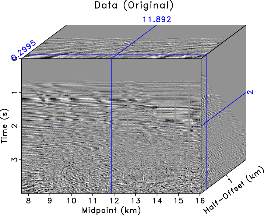
The fourth example is a numerically blended prestack field data. Figures 10a and 10b show the unblended and blended data that have been sorted from CSP gathers to CMP gathers. This example is used to simulate the independent marine-streamer simultaneous shooting (IMSSS) acquisition (Chen et al., 2014b). The blending interference is so strong that the useful reflections are nearly smeared in the noise. Figure 11a shows the velocity spectrum of the unblended data using the traditional semblance. Figure 11b shows the velocity spectrum of the blended data using the traditional semblance. Figure 11c shows the velocity spectrum of the blended data using the proposed high-resolution semblance. It is obvious that the traditional semblance can obtain good performance for clean unblended data. However, the traditional semblance cannot obtain a reasonable velocity spectrum for the blended data. Because of the strong blending interference, the traditional semblance cannot generate energy peaks in the spectrum that can be easily picked. Fortunately, the high-resolution similarity-weighted semblance can help obtain much focused peaks in the velocity spectrum that can be picked. With the automatically picked velocity (Fomel, 2009) from the velocity spectrum shown in Figure 11, we can obtain their corresponding migration results. Here, it is worth giving a brief introduction about the automatic velocity picking algorithm. Although the automatic velocity picking problem was mentioned by several researchers in the literature (Arnaud et al., 2004; Harlan, 2001; Adler and Brandwood, 1999; Sarkar and Baumel, 2000), we use the approach proposed in Fomel (2009). The main principle of the approach is to solve the following eikonal equation
The migrated profiles using the prestack kirchhoff time migration (PSKTM) algorithm for different cases are shown in Figure 12. Figure 12a shows the migrated profile for unblended data using the traditional semblance method. Figures 12b and 12c show the migrated profiles for blended data using the traditional semblance and the proposed high-resolution semblance, respectively. In this example, we can consider Figure 12a as the true answer, and judge the performance of different approaches by comparing the migrated results with Figure 12a. We can observe huge difference between Figures 12a and 12b. However, Figures 12a and 12c are more similar. We can confirm this observation by zooming a part from the original migrated profiles. Figure 13 shows the zoomed sections that correspond to the frame boxes shown in Figure 12. It is more obvious that Figures 13a and 13c show very similar reflections, while Figure 13b is much different from the other two cases. The erroneous reflections in Figure 13b indicate erroneous picked velocities using the traditional semblance.

|
|---|
|
simple-comp-dat
Figure 5. Synthetic data example. Left: Unblended CMP gather. Right: Blended CMP gather. |
|
|

|
|---|
|
simple-comp-scn
Figure 6. Left: Velocity spectrum of blended data using the conventional semblance. Right: Velocity spectrum of blended data using the high-resolution semblance. |
|
|

|
|---|
|
comp-dat
Figure 7. Field data example. Left: Unblended CMP gather. Right: Blended CMP gather. |
|
|

|
|---|
|
comp
Figure 8. Left: Velocity spectrum of unblended data using conventional semblance. Middle left: Velocity spectrum of unblended data using similarity-weighted semblance. Middle right: Velocity spectrum of blended data using the conventional semblance. Right: Velocity spectrum of blended data using the high-resolution semblance. |
|
|

|
|---|
|
comp2
Figure 9. (a) Blended CMP gather with strong blending interference. (b) Velocity spectrum using the conventional semblance. (c) Velocity spectrum using the high-resolution semblance. |
|
|

|
|---|
|
gulf,gulf-b
Figure 10. Gulf of Mexico data example. (a) Unblended field data. (b) Numerically simulated field data. |
|
|


|
|---|
|
vscan-gulf,vscan-b,vscan-simi-b
Figure 11. Comparison of velocity spectrum. (a) Velocity analysis of unblended data using the traditional approach. (b) Velocity analysis of blended data using the traditional approach. (c) Velocity analysis of blended data using the proposed approach. |
|
|


|
|---|
|
pstm,pstm-b,pstm-simi-b
Figure 12. Comparison of migration results. (a) PSKTM of unblended data using the traditional picked velocities. (b) PSKTM of blended data using the traditional approach. (c) PSKTM of blended data using the proposed approach. |
|
|


|
|---|
|
pstmzoom,pstm-bzoom,pstm-simi-bzoom
Figure 13. Comparison of zoomed migration results. (a) PSKTM of unblended data using the traditional approach. (b) PSKTM of blended data using the traditional approach. (c) PSKTM of blended data using the proposed approach. |
|
|
|
|
|
|
Velocity analysis of simultaneous-source data using high-resolution semblance - coping with the strong noise |