Automated spectral recomposition with application in stratigraphic interpretation

Stratigraphic interpretation

Setting the bandwidth for the frequency component ensures an accurate interpretation. Carrying valuable geological information, the main lobe of a wavelet has a finite duration, which means that it covers a certain range in the frequency domain. However, interpreters tend to pick a single frequency with bandpass filtering, which hardly covers the corresponding seismic information because a single frequency appears as a spike ignoring all other frequency content. Spectral recomposition helps in computation of frequency bandwidth of the main lobe. One can compute $t_d=\sqrt{6}/({f_m \pi})$ as in Figure 5, where $t_d$ is the dominant wavelength and $f_m$ is the peak frequency. The first zero crossing is computed as $t_r=t_d/\sqrt{3}$ (Sheriff, 2002). Having estimated the dominant wavelength, we can set the corresponding bandwidth in the frequency domain.

rkband
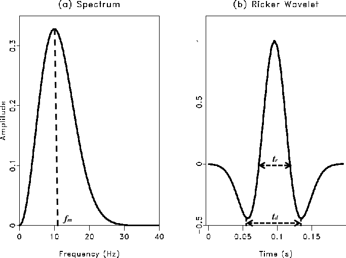
Figure 5. After extracting peak frequency $f_m$ , we compute the dominant wavelength and bandpass filter. (a) Spectrum with peak frequency $f_m$ . (b) Ricker wavelet with dominant wavelength $t_d$ and first zero crossing $t_r$ .

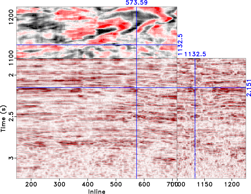
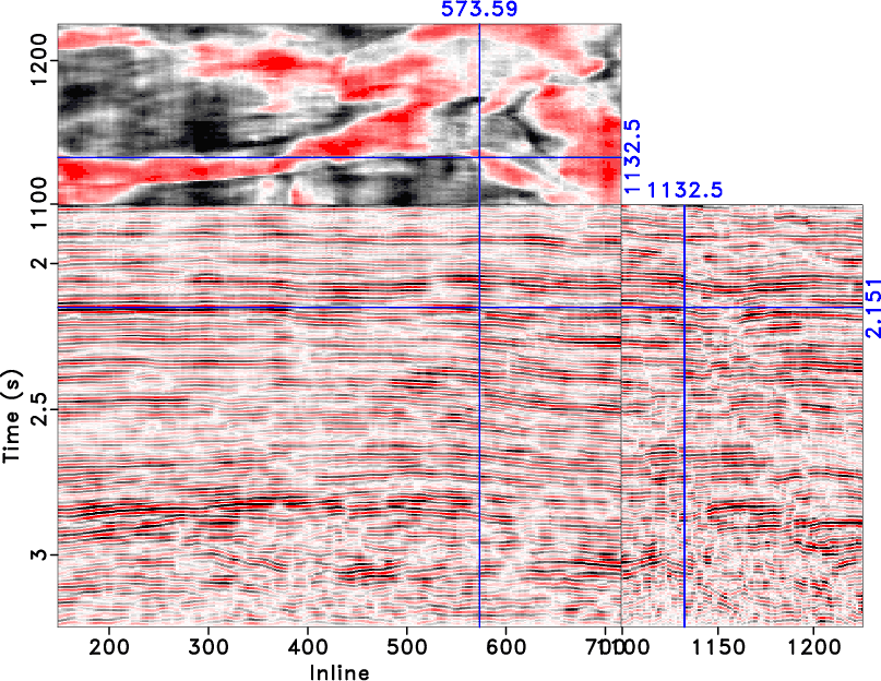
Spectral recomposition extracts significant components from seismic data. Picking the peak frequencies and setting their bandwidths produce results, as shown in Figures 6b and 6c. The same cross section is displayed with a manually picked peak frequency in Figure 6a. Note that Figures 6b and 6c reveal more geologic features. Reflections and seismic events are displayed better in Figure 6b and 6c; for example, a fault system clearly shows up in both Figure 6b and 6c, but not in Figure 6a. Deeper events are also well displayed in Figure 6c, but not in Figure 6a.

sgr330,sgr317,sgr321
Figure 6. (a) Seismic data from Starfak and Tiger Shoal field displayed with manually picked frequency bandpass filter. Using spectral recomposition, we display the same seismic data with two significant components in (b) and (c). A fault system between inline 800 to 900 clearly stands out in (b). Deep events below 2.4s are well displayed in (c). However, neither the fault system nor the deep events are well displayed in (a).

The concept behind spectral recomposition is that the seismic response of the geologic unit has a characteristic expression in the frequency domain that is indicative of its significant components (Tomasso et al., 2010). Hence, spectral recomposition can be used in time-slice or stratal-slice interpretation. We start by picking a depositional surface (geologic-time surface) so that any seismic attribute extracted on such a surface could represent a genetic depositional unit. Such a seismic surface display was termed a stratal slice (Zeng et al., 1998a,b). To showcase the ''recomposition'' technique developed here, we used data from Starfak and Tiger Shoal fields of offshore Louisiana, a 135-mile$^2$ 3-D survey area. The study area lies along the western periphery of the ancestral Mississippi River depocenter (McGookey, 1975), most recently designated the central Mississippi sediment-dispersal axis by Galloway et al. (2000).

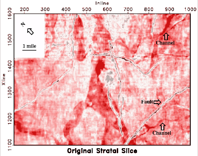
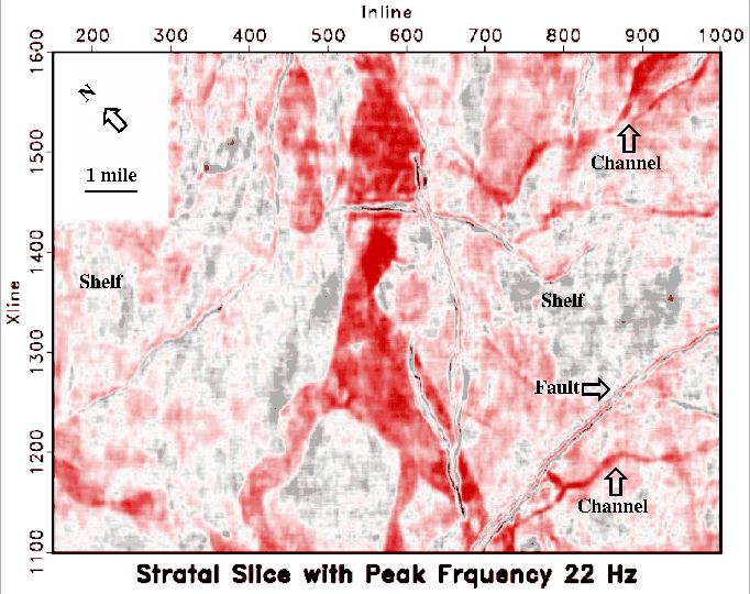
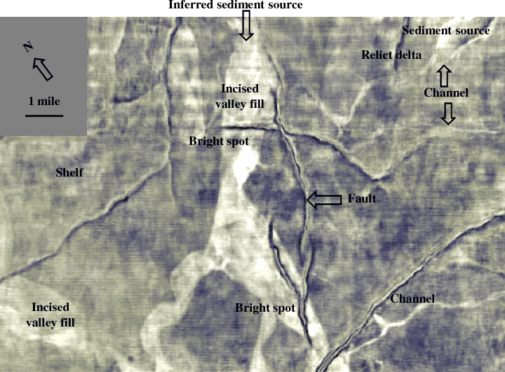
Zeng et al. (2001) constructed and interpreted stratal slices by using special tools to restore and refine multiple seismic slices in the wire-line-log context in both the traveltime domain and the relative geologic-time domain. Their approach includes conditioning seismic data to log lithology by $90^o$ phasing to achieve better well log integration, imaging, and interpretation of the sequential, planoform geomorphology of the depositional systems (Zeng and Backus, 2005). Our goal is to use spectral recomposition to further improve the image of seismic depositional facies; e.g. a high-frequency component helps indicate thin stratigraphic layers, while a low-frequency component helps identify thick stratigraphic layers. Depositional facies of different thickness can be differentiated using spectral recomposition. After extracting significant spectral components and setting band pass filters, we plotted the stratal slices of Starfak and Tiger Shoal field. Figure 7a is an upper Miocene-age horizon extracted by Zeng and Hentz (2004). Spectral recomposition shows that the component with 22 Hz peak frequency is a significant one, thus we have Figure 7b. As can be seen, Figure 7b improves imaging of the architectural elements within the depositional system. The thin, narrow channel sandstones in relict delta are more clearly imaged in Figure 7b than in Figure 7a. The shelf systems can be easily identified in Figure 7b but not in Figure 7a. Figure 7b is also less affected by acquisition footprint compared with Figure 7a. More than that, spectral recomposition works more efficiently. Both true time and thickness information has been extracted in the process. No prior time or depth-thickness estimate is required for automatic spectral recomposition.

After extracting significant signal components, the result of spectral recomposition naturally admits a Red-Green-Blue (RGB) color-blending plot. RGB color-blending plot takes advantage of the fact that human eyes can discriminate a large numbers of colors. One can plot horizontal slices of different frequency content in different colors, either red, green or blue, and combine them into one figure (Chopra and Marfurt, 2007). Picking frequency subsets automatically with solid geological and geophysical reasoning, spectral recomposition helps standardize the workflow of the RGB color-blending plot. As we have seen in Figure 3, spectral recomposition extracts dominant components at each time depth. Given a time slice or stratal slice, we extract the significant frequency components, compute the duration of the main lope of the wavelet from the area of interest, and set the appropriate bandwidth in the frequency domain. Plotting three different frequency components in RGB colors and combining them together, we produce RGB color-blending plots in Figure 8. With a sense of relative sandstone thickness distribution, RGB color blending of spectral recomposition brings useful information together and helps reveal geological features of interest.

slice0,slice1
Figure 7. Use of spectrum recomposition to improve thin-bed stratigraphic interpretation in Miocene, Starfak-Tiger Shoal fields, offshore Louisiana. (a) A stratal slice made by Zeng et al. (2001). (b) Same stratal slice extracted from 22 Hz component of seismic data.

rgb
Figure 8. Components of 15, 22, and 29 Hz of Starfak-Tiger Shoal stratal slice picked and plotted using color blending, which provides more detailed information. White bright colors indicate thicker sands; white dim colors refer to thinner sands; blue and dark colors indicate shale. Interpreters can easily identify different depositional facies in plot.

Automated spectral recomposition with application in stratigraphic interpretation