|
|
|
|
Plane-wave Sobel attribute for discontinuity enhancement in seismic images |
![\begin{displaymath}
S_i=\left[
\begin{array}{rrr}
-1 & 0 & 1 \\
-2 & 0 & 2 \\
...
...\right]\left[
\begin{array}{ccc}
-1 & 0 & 1
\end{array}\right]
\end{displaymath}](img4.png) |
(1) |
![\begin{displaymath}
S_x=S_i^{\mathrm{T}}=\left[
\begin{array}{rrr}
-1 & -2 & -1 \\
0 & 0 & 0 \\
1 & 2 & 1
\end{array}\right]
\end{displaymath}](img5.png) |
(2) |
In the ![]() -transform notation, filters (1) and (2) can be expressed as
-transform notation, filters (1) and (2) can be expressed as
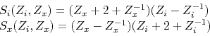 |
(3) |
where ![]() is a phase shift in the
is a phase shift in the ![]() direction.
direction.
The inline and crossline images are combined to approximate the magnitude of the image gradient (Chopra and Marfurt, 2007) where ![]() is the data and
is the data and ![]() and
and ![]() are convolution operators with the filters
are convolution operators with the filters ![]() and
and ![]() , respectively.
, respectively.
| (4) |
We propose to modify the filter for application to 3D seismic images by orienting the filter along the structure of seismic reflectors. Local slopes of seismic reflections are estimated in the inline and crossline directions using accelerated plane-wave destruction filters (Chen et al., 2013). The local-plane wave model assumes seismic traces can be effectively predicted by dynamically shifting adjacent seismic traces. This dynamic shift corresponds to the dip of seismic reflections. This model is useful for seismic data characterization and is the basis for plane-wave destruction filters. The local plane-wave differential equation is defined by Claerbout (1992) as
| (5) |
where ![]() is the seismic wavefield and
is the seismic wavefield and ![]() is the temporally and spatially variable local slope.
The optimal local slopes in the inline and crossline directions can be determined by minimizing the regularized plane-wave residual (Fomel, 2002; Chen et al., 2013).
is the temporally and spatially variable local slope.
The optimal local slopes in the inline and crossline directions can be determined by minimizing the regularized plane-wave residual (Fomel, 2002; Chen et al., 2013).
We further modify the Sobel filter by replacing the derivative operation with plane-wave destruction (Fomel, 2002) and the smoothing operation with plane-wave shaping (Fomel, 2007; Swindeman, 2015).
High order plane-wave destruction filters are described in the ![]() -transform notation as
-transform notation as
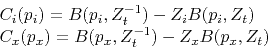 |
(6) |
where ![]() is the plane-wave destruction filter,
is the plane-wave destruction filter, ![]() is an all-pass filter, and
is an all-pass filter, and ![]() and
and ![]() are the local slopes in the inline and crossline directions, respectively.
are the local slopes in the inline and crossline directions, respectively.
Inline and crossline shaping filters are applied to the crossline and inline plane-wave destruction images, respectively.
Thus, the plane-wave Sobel filter modifies equation (3) by effectively replacing ![]() with
with
| (7) |
| (8) |
This modification effectively orients the plane-wave Sobel filter along seismic reflection structures.
In the conventional implementation, the inline and crossline images are combined to produce the final image (equation 4).
We propose an alternative approach based on the efficient azimuth scanning workflow (Merzlikin et al., 2017b).
We scan through a window of azimuths and compute the ![]() norm of linear combinations of the inline and crossline images weighted by the sine and cosine of the azimuth
norm of linear combinations of the inline and crossline images weighted by the sine and cosine of the azimuth ![]()
| (9) |
where
![]() and
and
![]() correspond to convolution operators with the filters
correspond to convolution operators with the filters ![]() and
and ![]() , respectively.
The azimuth which corresponds with the discontinuous features produces the best image at each point is picked on a semblance-like panel using a regularized automatic picking algorithm (Fomel, 2009).
In images with cross-cutting relationships between discontinuous geologic features, the azimuth which corresponds to the more prominent discontinuity will be preferentially selected.
The ensemble of images is then sliced using the pick to generate the optimal image.
This improves the resolution of discontinuous features by effectively orienting the plane-wave Sobel filter perpendicular to edges in the seismic image.
, respectively.
The azimuth which corresponds with the discontinuous features produces the best image at each point is picked on a semblance-like panel using a regularized automatic picking algorithm (Fomel, 2009).
In images with cross-cutting relationships between discontinuous geologic features, the azimuth which corresponds to the more prominent discontinuity will be preferentially selected.
The ensemble of images is then sliced using the pick to generate the optimal image.
This improves the resolution of discontinuous features by effectively orienting the plane-wave Sobel filter perpendicular to edges in the seismic image.
As suggested by equation (9), this workflow can be applied the seismic image ![]() ; however, we find that the azimuth of the seismic expression of discontinuous geologic features can be estimated more accurately by applying the workflow outlined above to a coherence, semblance, or Sobel filtered image.
In other words, we suggest to replace
; however, we find that the azimuth of the seismic expression of discontinuous geologic features can be estimated more accurately by applying the workflow outlined above to a coherence, semblance, or Sobel filtered image.
In other words, we suggest to replace ![]() in equation (9) with the plane-wave Sobel filter image (
in equation (9) with the plane-wave Sobel filter image (
![]() ).
By cascading multiple iterations of the plane-wave Sobel filter, we generate a more segmented image with less noise and improved estimates of the azimuth of the discontinuous features as expressed in the seismic image.
Instead of replacing
).
By cascading multiple iterations of the plane-wave Sobel filter, we generate a more segmented image with less noise and improved estimates of the azimuth of the discontinuous features as expressed in the seismic image.
Instead of replacing ![]() with the plane-wave Sobel filter image, we invite users to cascade their favorite coherence or semblance attributes with the plane-wave Sobel filter to further enhance discontinuous features in seismic images.
with the plane-wave Sobel filter image, we invite users to cascade their favorite coherence or semblance attributes with the plane-wave Sobel filter to further enhance discontinuous features in seismic images.
|
|
|
|
Plane-wave Sobel attribute for discontinuity enhancement in seismic images |