|
|
|
|
Random noise attenuation by a selective hybrid approach using f-x empirical mode decomposition |
The process of EMD is to gradually remove the stable oscillations embedded in the original signal and obtain a monotonic and smooth residual or trend at last. When it is applied to the seismic profile in each frequency slice along the spatial direction in the ![]() domain, the spatially-variant components, usually denoting the dipping events and random noise, will be gradually removed and the spatially-invariant components will be obtained as the residual at last. The small-dip-angle or exactly-horizontal events seismic profile can be considered as spatially invariant or spatially monotonic, thus they can be safely preserved no matter how many IMFs are removed in the frequency-slice decomposition process. On the other hand, the more IMFs are removed, the heavier damage of the dipping events will be caused.
domain, the spatially-variant components, usually denoting the dipping events and random noise, will be gradually removed and the spatially-invariant components will be obtained as the residual at last. The small-dip-angle or exactly-horizontal events seismic profile can be considered as spatially invariant or spatially monotonic, thus they can be safely preserved no matter how many IMFs are removed in the frequency-slice decomposition process. On the other hand, the more IMFs are removed, the heavier damage of the dipping events will be caused.
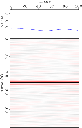
Figure 3 shows a demonstration of ![]() EMD for a flat-event synthetic section. In each panel, the upper graph is the real part of 20 Hz frequency slice, and the down profile is the corresponding synthetic section. The clean data, added Gaussian white noise, and noisy data are shown in Figures 3a, 3b and 3c, respectively. From the 20 Hz frequency slice we can see the flat event has zero spatial frequency. After
EMD for a flat-event synthetic section. In each panel, the upper graph is the real part of 20 Hz frequency slice, and the down profile is the corresponding synthetic section. The clean data, added Gaussian white noise, and noisy data are shown in Figures 3a, 3b and 3c, respectively. From the 20 Hz frequency slice we can see the flat event has zero spatial frequency. After ![]() EMD with 4 IMFs removed in each frequency slices, the denoised section is very clean, with the corresponding 20 Hz frequency slice nearly constant, the perfect denoising effect can be verified by looking at the removed noise section, where no coherent signal is found and the spectrum is nearly the same as that of the original added Gaussian white noise section.
EMD with 4 IMFs removed in each frequency slices, the denoised section is very clean, with the corresponding 20 Hz frequency slice nearly constant, the perfect denoising effect can be verified by looking at the removed noise section, where no coherent signal is found and the spectrum is nearly the same as that of the original added Gaussian white noise section.
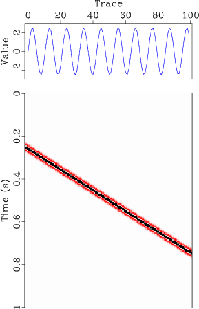
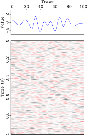
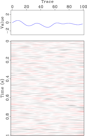
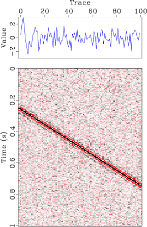
The perfect denoising performance does not hold for a dipping-event synthetic section, which is shown in Figure 4. According to the spectrum of the clean dipping event shown in Figure 4a, we know that a dipping event corresponds to a sine curve in the 20 Hz slice of the frequency domain. In this case, denoising performances corresponding to different number of removed IMFs are compared. Figures 4d, 4e and 4f shows the denoised section by removing 1, 2 and 3 IMFs, respectively. Figures 4g, 4h and 4i are corresponding noise sections. It's obvious that by removing only 1 IMF, the useful dipping signal has been harmed to a large extent. After removing 2 IMFs, most of the useful energy has been removed. Removing 3 IMFs removes totally the dipping event from the data section and the sine curve from the spectrum graph. For field seismic data that contains complex subsurface structure, ![]() EMD cannot be effective, which becomes its biggest issue.
EMD cannot be effective, which becomes its biggest issue.


|
|---|
|
flat-clean,flat-noise,flat-noisy,flat-denoised,flat-noise1
Figure 3. A demonstration of |
|
|


|
|---|
|
dip-clean,dip-noise,dip-noisy,dip-denoised1,dip-denoised2,dip-denoised3,dip-noise1,dip-noise2,dip-noise3
Figure 4. A demonstration of |
|
|


|
|---|
|
dip-mssa-denoised,dip-mssa-noise
Figure 5. A demonstration of |
|
|
|
|
|
|
Random noise attenuation by a selective hybrid approach using f-x empirical mode decomposition |