|
|
|
|
Fast dictionary learning for noise attenuation of multidimensional seismic data |
Next: Conclusion Up: Examples Previous: Synthetic example
|
|
|
|
Fast dictionary learning for noise attenuation of multidimensional seismic data |
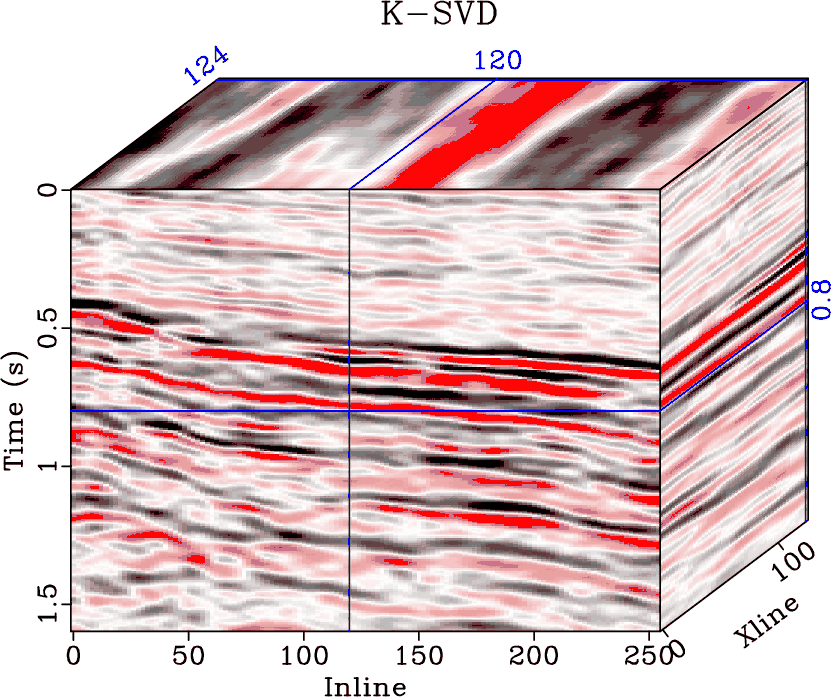
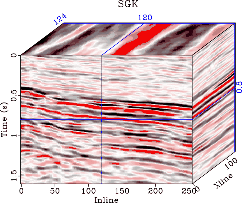
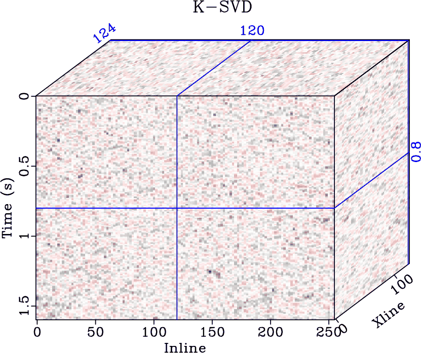
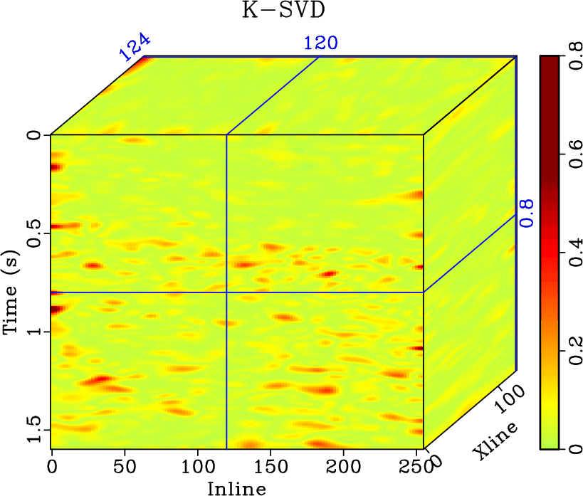
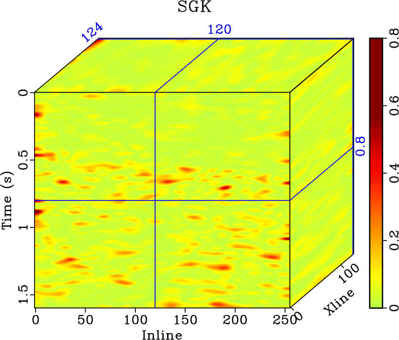
I next use a 3D field data example to demonstrate the performance, as shown in Figure 9. Figures 9a, 9b, and 9c show noisy data, K-SVD denoised data and SGK denoised data, respectively. Figures 9d and 9e show the noise sections of two approaches. It is clear that both approaches obtain approximate performance. It is computationally expensive to use K-SVD to learn the dictionary for this example. While it takes about half an hour to learn the dictionary using SGK algorithm, it takes more than half a day to learn the dictionary using the K-SVD algorithm. The local similarity cubes between denoised data cubes and removed noise cubes using two methods are shown in Figure 10, which confirms the successful and comparable performance of both methods in that most part of the data is close to zero.
|
|---|
|
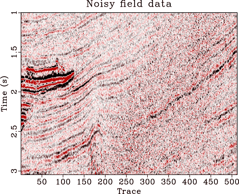
field2d
Figure 4. Noisy 2D field data. |
|
|

|
|---|
|
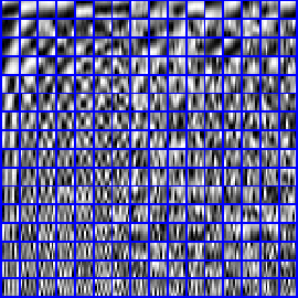
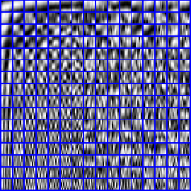
dicfield0,dicfieldksvd,dicfieldsgk
Figure 5. (a) Initial overcomplete DCT dictionary. (b) Learned dictionaries using K-SVD. (c) Learned dictionaries using SGK. Each atom in the dictionary has been reshaped into a 2D matrix. As can be seen in either (b) or (c) that there are some atoms in the middle part of the dictionary map containing linear patterns, indicating a better representation of the locally linear events. |
|
|


|
|---|
|
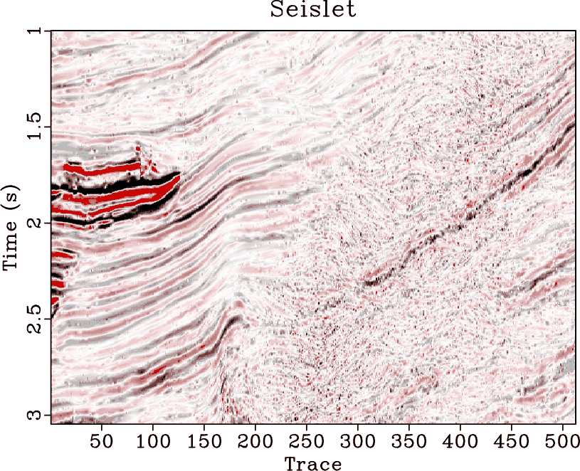
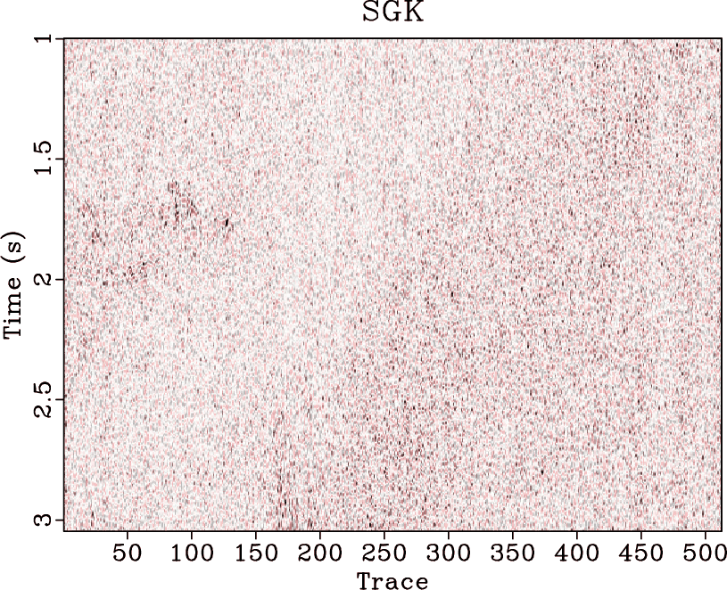
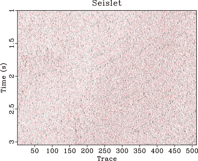
field2d-ksvd,field2d-sgk,field2d-ddtf,field2d-seis
Figure 6. (a) Denoised data using K-SVD. (b) Denoised data using SGK. (c) Denoised data using DDTF. (d) Denoised data using seislet thresholding. |
|
|


|
|---|
|
field2d-n-ksvd,field2d-n-sgk,field2d-n-ddtf,field2d-n-seis
Figure 7. (a) Removed noise using K-SVD. (b) Removed noise using SGK. (c) Removed noise using DDTF. (d) Removed noise using seislet thresholding. |
|
|


|
|---|
|
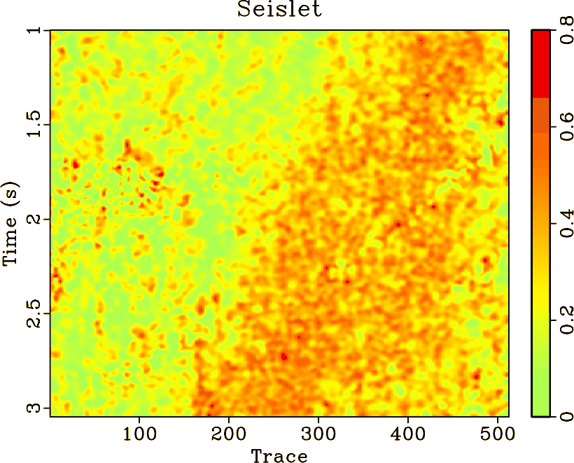
field2d-simi1,field2d-simi2,field2d-simi3,field2d-simi4
Figure 8. Local similarity between denoised data and removed noise using (a) K-SVD, (b) SGK, (c) DDTF and (d) seislet thresholding. |
|
|


|
|---|
|
field3d,field3d-ksvd,field3d-sgk,field3d-ksvd-n,field3d-sgk-n
Figure 9. (a) Noisy 3D field data. (b) & (c) Denoised data using K-SVD and SGK. (d) & (e) Noise cubes using K-SVD and SGK. |
|
|
|
|---|
|
field3d-simi1,field3d-simi2
Figure 10. (a) Local similarity between denoised data using K-SVD and the corresponding noise cube. (b) Local similarity between denoised data using SGK and the corresponding noise cube. |
|
|
|
|
|
|
Fast dictionary learning for noise attenuation of multidimensional seismic data |