 |
 |
 |
 | A parallel sweeping preconditioner for heterogeneous 3D Helmholtz equations |  |
![[pdf]](icons/pdf.png) |
Next: Global vector distributions
Up: Parallel sweeping preconditioner
Previous: Parallel multifrontal algorithms
Selective inversion
The lackluster scalability of dense triangular solves is well known and
a scheme known as selective inversion was introduced
in (32) and implemented in (31)
specifically to avoid the issue; the approach is
characterized by directly inverting every distributed dense triangular matrix
which would have been solved against in a normal multifrontal triangular solve. Thus, after performing selective inversion, every parallel dense triangular
solve can be translated into a parallel dense triangular matrix-vector multiply.
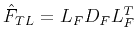
Suppose that we have paused a multifrontal  factorization just before
processing a particular front,
factorization just before
processing a particular front,  , which corresponds to some supernode,
 . Then all of the fronts for the descendants of
have already been handled, and
can be partitioned as
. Then all of the fronts for the descendants of
have already been handled, and
can be partitioned as
 |
(6) |
where  holds the Schur complement of supernode
with
respect to all of its descendants,
holds the Schur complement of supernode
with
respect to all of its descendants,  represents the coupling of
and its descendants to
's
ancestors, and
represents the coupling of
and its descendants to
's
ancestors, and  holds the Schur complement updates from
the descendants of
for the ancestors of
. Using
hats to denote input states, e.g.,
holds the Schur complement updates from
the descendants of
for the ancestors of
. Using
hats to denote input states, e.g.,
 to denote the input state
of
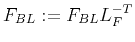
, the first step in processing the frontal matrix
is to
overwrite
with its
factorization, which is to say that
is overwritten with the strictly lower portion of a unit lower
triangular matrix
to denote the input state
of
, the first step in processing the frontal matrix
is to
overwrite
with its
factorization, which is to say that
is overwritten with the strictly lower portion of a unit lower
triangular matrix  and a diagonal matrix
  such that
 .
.
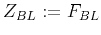
The partial factorization of
can then be completed via the following steps:
- Solve against
 to form
 .
.
- Form the temporary copy
 .
.
- Finalize the coupling matrix as
 .
.
- Finalize the update matrix as
 .
.
After adding
onto the parent frontal matrix, only
and
are needed in order to perform a multifrontal solve. For instance, applying
 to some vector
  proceeds up the elimination tree
(starting from the leaves) in a manner similar to the factorization;
after handling all of the work for the descendants of some supernode
, only a few dense linear algebra operations with
's
corresponding frontal matrix, say
, are required.
Denoting the portion of
corresponding to the degrees of freedom in
supernode
by
proceeds up the elimination tree
(starting from the leaves) in a manner similar to the factorization;
after handling all of the work for the descendants of some supernode
, only a few dense linear algebra operations with
's
corresponding frontal matrix, say
, are required.
Denoting the portion of
corresponding to the degrees of freedom in
supernode
by
 , we must perform:
-
-
- Add
 onto the entries of
corresponding to the parent supernode.
onto the entries of
corresponding to the parent supernode.
The key insight of selective inversion is that,
if we invert each distributed dense unit lower triangular matrix
in
place, all of the parallel dense triangular solves in a multifrontal
triangular solve are replaced by parallel dense matrix-vector multiplies. It
is also observed in (32) that the work required for the
selective inversion is typically only a modest percentage of the work required
for the multifrontal factorization, and that the overhead of the selective
inversion is easily recouped if there are several right-hand sides to solve
against.
Since each application of the sweeping preconditioner requires two multifrontal
solves for each of the
 subdomains, which are relatively small
and likely distributed over a large number of processes, selective inversion
will be shown to yield a very large performance improvement.
We also note that, while it is widely believed that direct inversion is
numerically unstable, in (11) Druinsky and Toledo
provide a review of (apparently obscure) results dating back to Wilkinson
(in (42)) which show that
subdomains, which are relatively small
and likely distributed over a large number of processes, selective inversion
will be shown to yield a very large performance improvement.
We also note that, while it is widely believed that direct inversion is
numerically unstable, in (11) Druinsky and Toledo
provide a review of (apparently obscure) results dating back to Wilkinson
(in (42)) which show that
 is
as accurate as a backwards stable solve if reasonable assumptions are met
on the accuracy of
is
as accurate as a backwards stable solve if reasonable assumptions are met
on the accuracy of
 . Since
 is argued to
be more accurate when the columns of
have been computed
with a backwards-stable solver, and both
is argued to
be more accurate when the columns of
have been computed
with a backwards-stable solver, and both
 and
and
 must be applied after selective inversion, it might
be worthwhile to modify selective inversion to compute and store two different
inverses of each
: one by columns and one by rows.
must be applied after selective inversion, it might
be worthwhile to modify selective inversion to compute and store two different
inverses of each
: one by columns and one by rows.
|
|
|
|
| A parallel sweeping preconditioner for heterogeneous 3D Helmholtz equations | |
|
Next: Global vector distributions
Up: Parallel sweeping preconditioner
Previous: Parallel multifrontal algorithms
2014-08-20