|
|
|
|
A parallel sweeping preconditioner for heterogeneous 3D Helmholtz equations |
Our experiments took place over five different 3D velocity models:
In all of the following experiments, the shortest wavelength of each model is resolved with roughly ten grid points and the performance of the preconditioner is tested using the following four forcing functions:
The first experiment was meant to test the convergence rate of the sweeping
preconditioner over domains spanning 50 wavelengths in each direction
(resolved to ten points per wavelength) and each test made use of 256 nodes of
Lonestar. During the course of the tests, it was noticed that a significant
amount of care must be taken when setting the amplitude of the derivative of
the PML takeoff function (i.e., the ``C'' variable in Eq. (2.1)
from (15)). For the sake of brevity, hereafter we refer to
this variable as the PML amplitude. A modest search was performed in
order to find a near-optimal value for the PML amplitude for each problem.
These values are reported in Table 1 along with the number
of iterations required for the relative residuals for all four forcing functions
to reduce to less than ![]() .
.
|
|---|
|
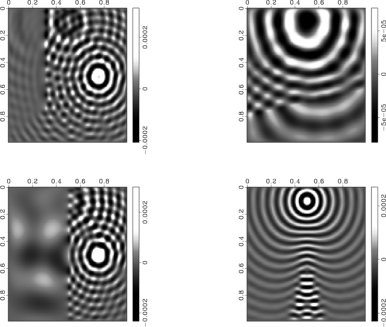
solution-models
Figure 5. A single |
|
|
It was also observed that, at least for the waveguide problem,
the convergence rate would be significantly improved if 6 grid points of PML
were used instead of 5.
In particular, the 52 iterations reported in Table 1 reduce
to 27 if the PML size is increased by one.
Interestingly, the same number of iterations
are required for convergence of the waveguide problem at half the frequency
(and half the resolution) with five grid points of PML. Thus, it appears that
the optimal PML size is a slowly growing function of the
frequency.We also note that, though it was not intentional, each of the these first four
velocity
models is invariant in one or more direction, and so it would be straightforward
to sweep in a direction such that only ![]() panel factorizations would need
to be performed, effectively reducing the complexity of the setup phase to
panel factorizations would need
to be performed, effectively reducing the complexity of the setup phase to
![]() .
.
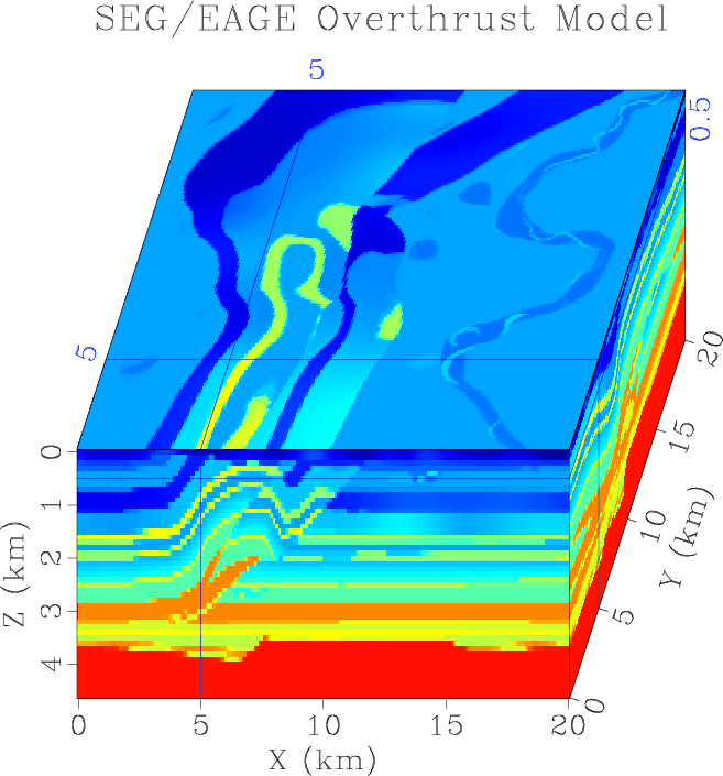
The last experiment was meant to simultaneously test the convergence rates and scalability of the new sweeping preconditioner using the Overthrust velocity model (see Fig. 9) at various frequencies, and the results are reported in Table 2. It is important to notice that this is not a typical weak scaling test, as the number of grid points per process was fixed, not the local memory usage or computational load, which both grow superlinearly with respect to the total number of degrees of freedom. Nevertheless, including the setup phase, it took less than three minutes to solve the 3.175 Hz problem with four right-hand sides with 128 cores, and just under seven and a half minutes to solve the corresponding 8 Hz problem using 2048 cores. Also, while it is by no means the main message of this paper, the timings without making use of selective inversion are also reported in parentheses, as the technique is not widely implemented.
|
|---|
|
overthrust
Figure 6. Three cross-sections of the SEG/EAGE Overthrust velocity model, which represents an artificial |
|
|
|
|---|
|
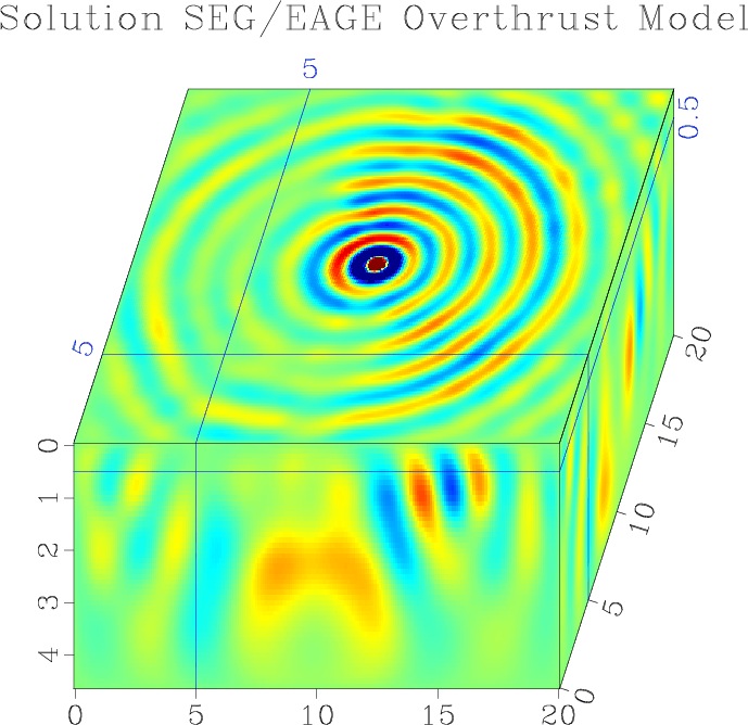
solution-overthrust
Figure 7. Three planes from a solution with the Overthrust model with a single localized shot at the center of the |
|
|
|
|
|
|
A parallel sweeping preconditioner for heterogeneous 3D Helmholtz equations |