|
|
|
|
A probabilistic approach to seismic diffraction imaging |

|
|---|
|
prob-dimage-flow
Figure 1. Probabilistic diffraction imaging workflow |
|
|

|
|---|
|
toy-data
Figure 2. Toy model data containing two reflectors and a point diffractor. |
|
|

|
|---|
|
toy-ovc-box
Figure 3. Example of application of OVC to toy model for three continuation velocities: left panel is under-migration with |
|
|
The process of OVC is applied to the data and their slope-decomposed images are propagated through a range of migration velocities to create a series of slope decomposed partial images. Slices through this volume are illustrated in Figure 3. The front panes of box plots in this figure display slope gathers centered at 0.5 km, directly above the diffractor, for three different migration velocities. The right right panes show the image created by stacking over slope for the selected migration velocity. Notice that for all three velocities, energy corresponding to the reflectors, near 2.1 s and 4 s, bend upward in the slope gathers. The lowest point in the upward bending reflection energy corresponds to the slope of that reflector. Notice that this apex is achieved at greater time values with higher migration velocities for the dipping reflector, and that the slope corresponding to this apex is greater for higher migration velocities. This is because migration makes dipping events steeper, and migration with larger velocities further increases the slope of dipping events. Diffraction energy in the left panel bends upward in a ``smile'' indicating under-migration. The energy flattens in the middle panel corresponding to correct migration. In the right panel it bends downward in a ``frown'' indicating over-migration. As we will see, the flat, correctly migrated diffraction energy results in a semblance high. Examining the stacked continuation images on the right panes of the box plots, we see that the diffraction bows downward when undermigrated in the left panel, is focused into a point when properly migrated in the center panel, and bows upward when overmigrated in the right panel. The slope of the dipping reflector increases with increased velocity, while the flat reflector's slope and vertical position is unaffected.
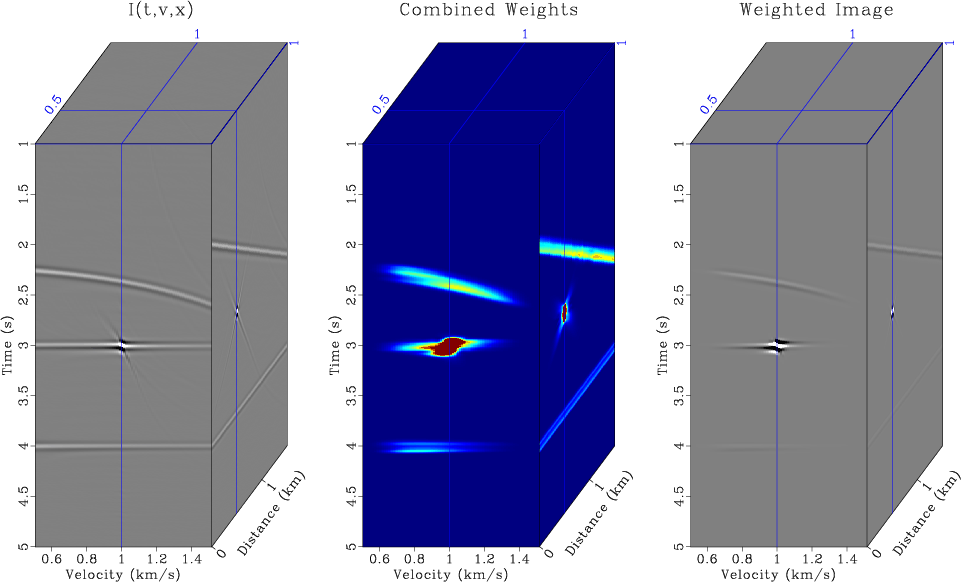
The creation and application of probabilistic weights to partial images images to create a probabilistic diffraction image is illustrated in Figure 4. The front pane of the top left box in Figure 4 contains a partial image in velocity generated by stacking the OVC output over slope at 0.5 km, centered directly above the diffractor, while the side pane shows the slice through this continuation volume for a velocity of 1 km/s, which corresponds to a deterministic image with the true migration velocity.
|
|---|
|
toy-weights3-1-a
Figure 4. Probabilistic migration process illustrating the action of weights on |
|
|
For this section we calculate the three imaging weights, shown in the bottom row of Figure 4. The bottom left box contains ![]() , the image semblance calculated according to Equation 3. Semblance provides a measure of when slope-gathers are flat, and thus semblance highs can indicate where diffractions have been migrated using the correct velocity. Using this semblance, the expectation velocity,
, the image semblance calculated according to Equation 3. Semblance provides a measure of when slope-gathers are flat, and thus semblance highs can indicate where diffractions have been migrated using the correct velocity. Using this semblance, the expectation velocity, ![]() , and its variance,
, and its variance,
![]() , are calculated according to Equations 4 and 5. A normal distribution is fit to that velocity and variance according to Equation 6, generating
, are calculated according to Equations 4 and 5. A normal distribution is fit to that velocity and variance according to Equation 6, generating ![]() which is plotted in the lower middle box.
which is plotted in the lower middle box.
Notice that ![]() , the expectation velocity, occurring at the maximum value of
, the expectation velocity, occurring at the maximum value of ![]() , does not track the true velocity,
, does not track the true velocity, ![]() km/s in the shallow or deep portions of the panel. This is because diffraction data does not exist there to be utilized for maximizing semblance. However,
km/s in the shallow or deep portions of the panel. This is because diffraction data does not exist there to be utilized for maximizing semblance. However,
![]() km/s at 3 s, where the diffraction takes place. The lower right box displays
km/s at 3 s, where the diffraction takes place. The lower right box displays ![]() , a weight based on how quickly semblance, or
, a weight based on how quickly semblance, or ![]() , changes in space.
, changes in space.
The three weights in the lower row of Figure 4 posses high values at the time and position of the diffraction at the correct migration velocity but they are also non-zero at other locations where diffraction did not occur. The top middle box of Figure 4 shows how multiplying the three weights together further emphasizes the region of the partial image with diffraction data. Multiplying this combined weight by the input ![]() in the top left box of Figure 4 generates the weighted partial image on the top right box of that Figure. Notice how the energy of the diffraction at the correct velocity is emphasized, while other energy present is suppressed.
in the top left box of Figure 4 generates the weighted partial image on the top right box of that Figure. Notice how the energy of the diffraction at the correct velocity is emphasized, while other energy present is suppressed.


|
|---|
|
toy-drefl,toy-det-img,toy-pathint-img,toy-prob-dimage
Figure 5. Comparison of probabilistic diffraction imaging output with other methods: (a) ideal image corresponding to the toy model reflectivity convolved with a 10 Hz peak frequency Ricker Wavelet; (b) deterministic image created by migrated the data in Figure 2 using its migration velocity, 1 km/s; (c) equal weight image generated by stacking |
|
|
We generate a suite of images to compare different imaging methods. Figure 5a contains an ``ideal image'' generated by convolving the toy model reflectivity with a 10 Hz peak frequency Ricker wavelet. Figure 5b contains the deterministic image created through migration with the correct velocity. Figure 5c contains an equal weight comparison image, constructed in the manner of the equal weight images featured in Merzlikin and Fomel (2017). This is the equivalent of stacking the top left box of Figure 4 over velocity for each midpoint. Figure 5d contains our probabilistic diffraction image, generated by stacking the weighted images shown in the top right box of Figure 4 over velocity for every midpoint. It is the output of Equation 8.
To highlight the wavefield components contributing to each of these images we generate a series of slope gathers centered above the diffractor at 0.5 km. Stacking each of these gathers over slope would create the traces at ![]() km in their corresponding images. Figure 6a contains an ``ideal gather'' generated by warping the ideal image in Figure 5a to squared time, decomposing it into constituent slope components, and warping the slope decomposed image back to time. The plane wave destruction slope calculated from the ideal image warped to squared time is plotted on this gather with fuchsia x's where reflectors are present. Figure 6b contains a gather contributing to the deterministic image, Figure 5b. This gather is generated by selecting
km in their corresponding images. Figure 6a contains an ``ideal gather'' generated by warping the ideal image in Figure 5a to squared time, decomposing it into constituent slope components, and warping the slope decomposed image back to time. The plane wave destruction slope calculated from the ideal image warped to squared time is plotted on this gather with fuchsia x's where reflectors are present. Figure 6b contains a gather contributing to the deterministic image, Figure 5b. This gather is generated by selecting
![]() for
for
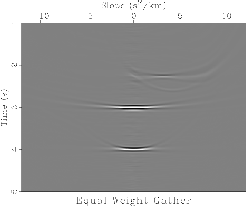
![]() km/s. Figure 6c contains a gather corresponding to the equal weight image, Figure 5c. It is constructed by stacking the slope decomposed partial images in velocity,
km/s. Figure 6c contains a gather corresponding to the equal weight image, Figure 5c. It is constructed by stacking the slope decomposed partial images in velocity,
![]() , over velocity. Figure 6d contains a gather corresponding to the probabilistic diffraction image, Figure 5d. It is generated by multiplying the combined weights and the slope decomposed partial images in velocity and stacking over velocity.
, over velocity. Figure 6d contains a gather corresponding to the probabilistic diffraction image, Figure 5d. It is generated by multiplying the combined weights and the slope decomposed partial images in velocity and stacking over velocity.


|
|---|
|
toy-ideal-gather-slope-1,toy-pick-gather-1,toy-const-gather-1,toy-wtd-gather-1
Figure 6. Slope gathers centered at 0.5 km, directly above the diffractor, corresponding to the: (a) ideal image, Figure 5a overlaid by slope denoted using fuchsia x's where reflectors are present; (b) deterministic image, Figure 5b; (c) equal weight image, Figure 5c; (d) the probabilistic diffraction image, Figure 5d. |
|
|
As one would expect, the ideal image in Figure 5a features excellently focused and easily discernible diffraction and reflection events. The diffraction in this image is marked by a well defined single point without features radiating away from that point - the point spread function is not present for the diffractor, as the Hessian corresponding to modeling and migration has not been applied to this image.
Examining the gather centered at ![]() km for this image, Figure 6a, the most visible feature is the energetic flat diffraction event extending across all slopes in the gather. One may think of two equivalent reasons for why diffraction energy appears this way in slope gathers. The first is because a point contains information from all slopes - one may see this by taking the
km for this image, Figure 6a, the most visible feature is the energetic flat diffraction event extending across all slopes in the gather. One may think of two equivalent reasons for why diffraction energy appears this way in slope gathers. The first is because a point contains information from all slopes - one may see this by taking the ![]() transform of a dot. The second is that if we think of an idealized diffraction hyperbola extending to infinity, that hyperbola will contain all slopes, from asymptotically vertical up to the right, to flat at the point of the diffractor, to asymptotically vertical downward to the right. Migration with the correct velocity collapses diffraction hyperbolas to a point. Thus a properly migrated idealized diffraction will contain information from all slopes transformed to the same point in space, and such a diffraction in a slope gather immediately above the diffractor would appear as a flat event extending over all slopes. In practice, even in synthetic experiments, seismic data does does not contain such idealized diffraction hyperbolas extending to infinity due to limited spatial geophone or receiver coverage, so only a portion of slopes contribute to the diffraction image. This effect is visible in the point spread function, appearing like a ``bow tie''. The two reflectors are also visible in this ideal gather, featuring energy confined to a narrower range of slopes centered about the observed slope for each reflector, noted by fuchsia x's. This is intuitive, because planar reflection events contain energy from their dominant slope.
transform of a dot. The second is that if we think of an idealized diffraction hyperbola extending to infinity, that hyperbola will contain all slopes, from asymptotically vertical up to the right, to flat at the point of the diffractor, to asymptotically vertical downward to the right. Migration with the correct velocity collapses diffraction hyperbolas to a point. Thus a properly migrated idealized diffraction will contain information from all slopes transformed to the same point in space, and such a diffraction in a slope gather immediately above the diffractor would appear as a flat event extending over all slopes. In practice, even in synthetic experiments, seismic data does does not contain such idealized diffraction hyperbolas extending to infinity due to limited spatial geophone or receiver coverage, so only a portion of slopes contribute to the diffraction image. This effect is visible in the point spread function, appearing like a ``bow tie''. The two reflectors are also visible in this ideal gather, featuring energy confined to a narrower range of slopes centered about the observed slope for each reflector, noted by fuchsia x's. This is intuitive, because planar reflection events contain energy from their dominant slope.
The deterministic image in Figure 5b appears similar to the ideal image in Figure 5a with an added ``bow tie'' point spread function around the diffractor. This result is unsurprising - it assumes complete apriori information about the subsurface velocity field. Differences with the ideal image are caused by the incomplete spatial sampling of the wavefield. Examining the gather corresponding to this image, Figure 6b shows that as was the case in the ideal gather, three clearly defined events are visible correlating to the two reflections, each centered at their corresponding slope, and the diffraction event. As is expected in such a synthetic experiment, the reflection and diffraction events for this deterministic gather generated using the correct migration velocity appear quite similar to those in the ideal gather. A minor difference between the two gathers is the appearance of upward bowing energy around reflection events in the deterministic gather, which is absent from the ideal gather. Also, notice that energy corresponding to the diffraction event increases for large amplitude slope values in the ideal gather, but remains relatively constant in the deterministic gather. This is a result of the slope decomposition used to generate the ideal gather placing diffraction energy for slopes larger than those present in the gather at those large slope values. A true ``ideal gather'' of a diffraction would have slopes extending to infinity and feature constant energy for all slope values.
In the equal weight image, Figure 5c, the flat reflector is imaged quite well, as all its energy is stationary at the correct time. The dipping reflector appears more smeared because the time its energy achieves the stationary apex in Figure 3 changes with velocity, and thus interferes destructively on stacking in this imaging method. The stationary remaining energy corresponds to that of the initial and final velocities, which have no lower or higher velocities respectively to interfere destructively with. This is evident in the gather corresponding to the equal weight image, Figure 6c, where two weak events corresponding to the dipping reflector are visible. The upper event is related to migration with the initial velocity, and the weaker, lower event is related to migration with the greatest velocity considered. This type of behavior can also be seen in the equal weight diffraction featured in Figure 5c. Rather than having a artifact around the diffraction corresponding to limited spatial coverage, as was the case in Figure 5b, here there is an artifact around the diffraction corresponding to only considering a limited set of migration velocities prior to stacking. Two events, a stronger one bowing downward which is an imprint left by undermigration of diffraction energy with the initial velocity, and a weaker upward bowing event corresponding to diffraction overmigration appear. If we performed this experiment using a dense sampling of velocities spanning all positive numbers, these artifacts would not be present. Diffraction energy is less well spatially resolved than in Figure 5b, appearing more laterally spread out.
The probabilistic diffraction image, Figure 5d successfully highlights diffraction energy and suppresses energy corresponding to reflectors. A ``bow tie'' point spread function similar to that appearing in Figure 5b is not present in this image, although there is a minor artifact appearing like a weaker version of the one surrounding the diffraction in Figure 5c. The diffraction in Figure 5d has similar lateral resolution to that in Figure 5b and superior resolution to Figure 5c. Examining the gather corresponding to the probabilistic diffraction image, Figure 6d, shows that although energy corresponding to the two reflection events is present, it is dramatically reduced compared to the deterministic gather in Figure 6b. This illustrates why the method is intended to be used on data where diffraction extraction has already been attempted - although reflection suppression has occurred it is not complete, so applying the method to complete data featuring both strong reflections and diffractions would not generate ideal results. However, this suppression is complementary to any data-domain reflection removal that occurs before applying the approach, for example using plane-wave destruction. Diffraction energy in the probabilistic gather appears flat, resembling the diffraction energy in the ``ideal gather'' of Figure 6a and the deterministic gather of Figure 6b, although the slope coverage of the probabilistic gather is more limited than those two. This is because diffraction energy present at large slopes is more responsive to velocity perturbation than those at small slopes, so destructive interference from partial images in velocity near the true migration velocity which receive a non-zero weight in the probabilistic imaging process suppress diffraction energy at these slope values.
|
|
|
|
A probabilistic approach to seismic diffraction imaging |