Numerical examples

Our first synthetic example consists of four isolated passive seismic events in a constant velocity (1.5km/s) media, shown in Figure 1 The sources are activated at 0.5s, 0.6s, 0.8s and 0.9s, from left to right. Amplitudes of the sources increase from left to right. Note that the 2nd source (0.6s) and 3rd source (0.8s) are aligned at the same depth in the model, they appear shifted in the seismic recording because of their activation time lag.

data-simple
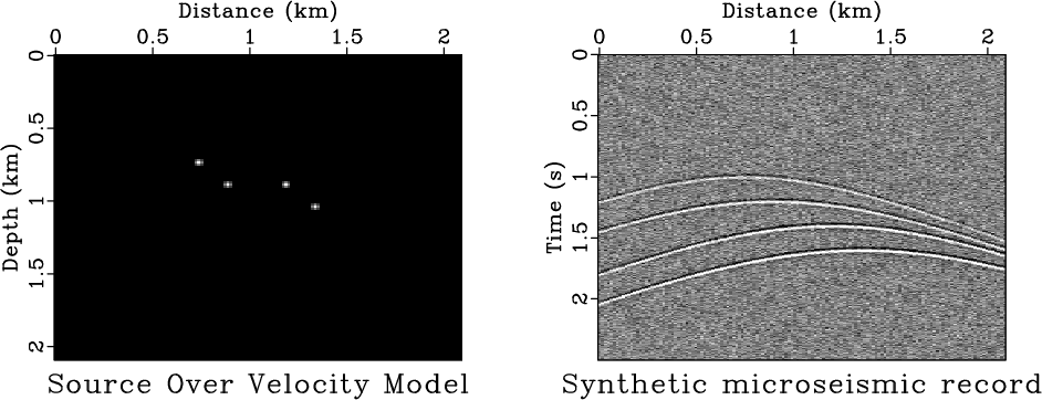
Figure 1. Synthetic microseismic model (left) and forward modeling data (right). Sources are activated at 0.5s, 0.6s, 0.8s, 0.9s,respectively from left to right. Amplitudes of the sources increase from left to right.

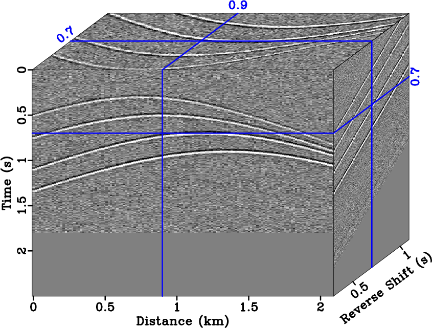
Figure 2 shows the construction of reverse-shifted hypercube. Data is sprayed to an extended dimension—reverse-time shift, then shifted along the time axis and padded after recording time. The time shift compensates for activation time lag of the passive seismic events. Migration can be performed on each $t$-$x$ slice of this data hypercube.

shift
Figure 2. Shifted data hypercube. Data is sprayed on another reverse-shift dimension, then shifted on each slice corresponding to the reverse-shift value.

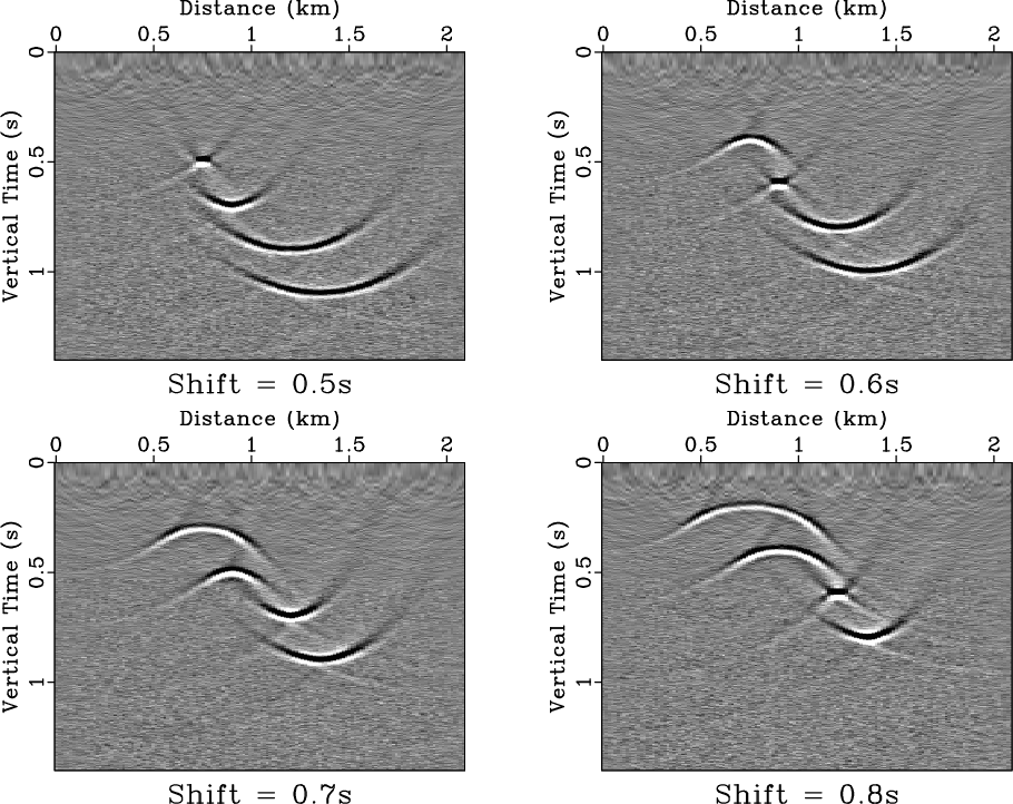
After processing with proposed path-integral time-domain diffraction imaging on the extended dataset $D(t,x,\tau)$, some slices of the image volume 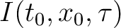$I(t_0,x_0,\tau )$ are shown in Figure 3. The path-integral migration only requires velocity limits (maximum and minimum values of velocity) instead of detailed velocity model estimation; for this constant velocity model, we add 0.3km/s of velocity uncertainty in the migration. At the delay times corresponding to the true activation times (0.5s, 0.6s and 0.8s), the sources focus at their true locations; at other incorrect activation time (0.7s), no event focuses.

act
Figure 3. Passive seismic energy focus, corresponding to their true on sets, at their locations.

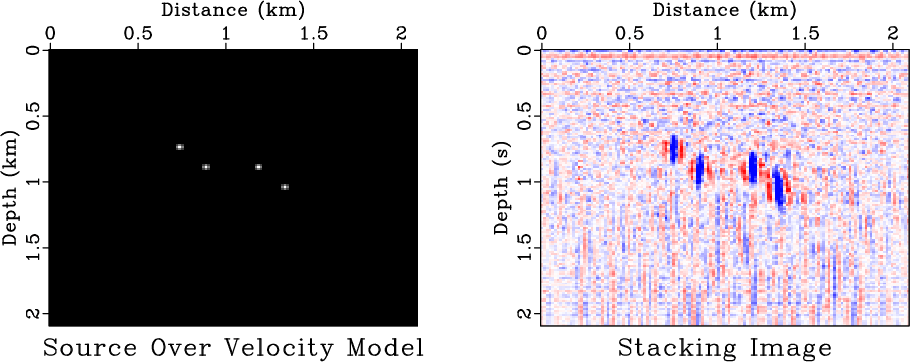
Using amplitude envelope stacking, Laplacian sharpening and then converting to depth coordinates, a stacking image of source localizations is shown in Figure 4 with comparison between the true model and time-domain migration image. Although noise contaminates localization image, the four sources are easy to identify as a clear pattern. The spatial localizations match the sources locations in the synthetic model.

migstack-simple
Figure 4. Microseismic imaging result of first synthetic example. Comparison between (left) synthetic model and (right) microseismic imaging after envelope stacking and Laplacian sharpening.

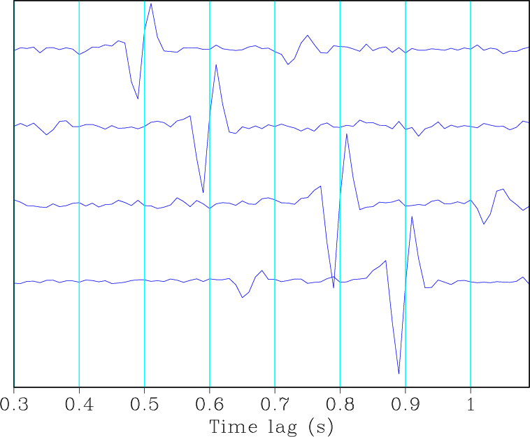
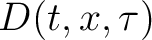
In the image in Figure 4, we can pick four sources' spatial locations; another task is to determine their activation times. Extracting the time-shift traces from image volume $I(t_0,x_0,\tau )$ at four picked sources positions, the traces are shown in Figure 5. From the upper to the lower part, the wavelets in the trace indicates onsets of the corresponding source. The temporal activation times match the onsets in the model.

trc
Figure 5. Four traces extracted from image volume $I(t_0,x_0,\tau )$ at four picked source positions.

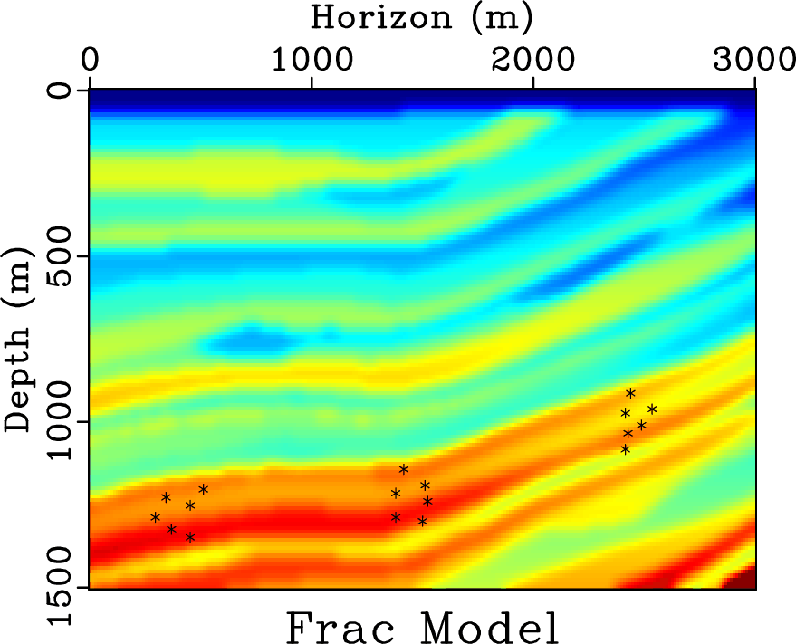
Our next example includes a more complicated velocity model, cropped from the Marmousi model (Versteeg, 1994) to test the stability of the proposed time-migration method in the presence of velocity heterogenities. Figure 6 demonstrates this synthetic model. The sources are divided into three groups, activated from left to right, resembling the three stages of fracture growth in hydraulic fracturing.

sov
Figure 6. Source locations over velocity model. Three groups subsurface microseismic sources are activated from left to right. This is similar to the three stages of fracture system growth in hydraulic fracturing.

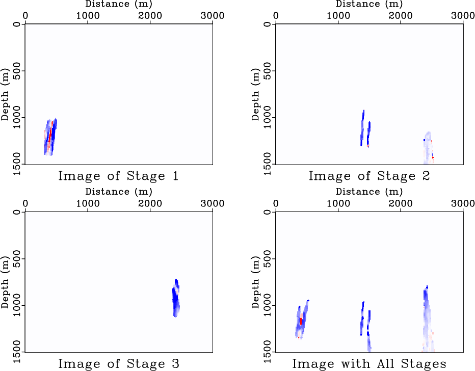
Instead of stacking along all reverse-shift values, stacking can also be performed within a sliding time window that includes certain stages of the injection. Figure 7 is the stacking image within the first, second, third stage and the full range of injection, respectively. We applied thresholding after envelope stacking and converted time-coordinate images to depth coordinates using the same velocity model for comparison. Microseismic events activated at the corresponding stage are focused, while other events that are not activated in this stage are defocused and suppressed after envelope stacking. Stacking image over full range shows all three stages of sources.

migstack
Figure 7. Stacking images over first, second and third stage of injection and full range of reverse-time shifting.

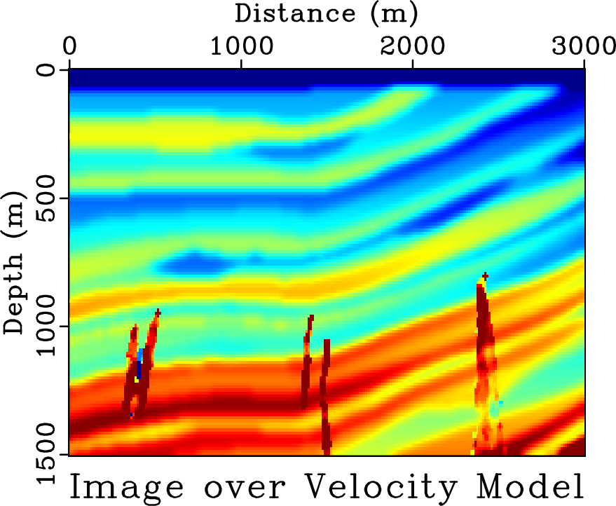
Figure 8 shows the stacking image over full range of stages superimposed on the velocity model.

mig-vel
Figure 8. Microseismic imaging with full range of stages, superimposed on velocity model.