|
|
|
|
Microseismic source localization using time-domain path-integral migration |
Next: Imaging condition: envelope stacking Up: Methodology Previous: Methodology
|
|
|
|
Microseismic source localization using time-domain path-integral migration |
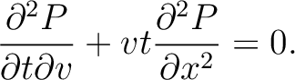
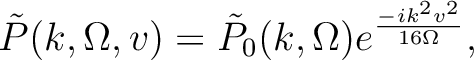
 , the solution for equation 1 can be expressed as (Fomel, 2003a):
where
, the solution for equation 1 can be expressed as (Fomel, 2003a):
where  is migration velocity,
  is the Fourier dual of
  and
and  is wavenumber.
The input zero-offset stack
is wavenumber.
The input zero-offset stack
 is transformed to a constant velocity time migrated image
 .
Burnett and Fomel (2011) provide an extension to the 3-D anisotropic case.
.
Burnett and Fomel (2011) provide an extension to the 3-D anisotropic case.
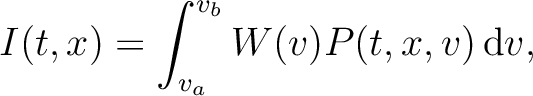
The path-integral formulation creates velocity independent images (Landa et al., 2006) in time domain; the formulation of velocity-weighted path-integral of VC images is:
where is the velocity-weighting function used to fine-tune velocity constraints formed by
  and
and  .
.
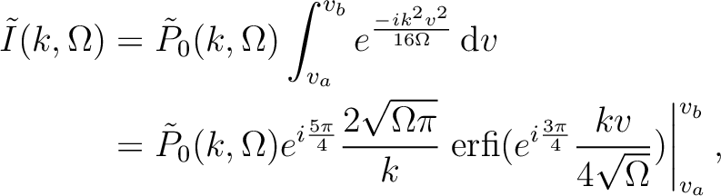
Efficient workflow of the integral above, proposed by Merzlikin and Fomel (2015), is integrating velocity analytically in the double-Fourier domain. For example, an unweighted integral takes the form:
which turns path-integral into an analytical filter in double-Fourier domain. Velocity-weighting function with analytical forms can be included also in this integral.The efficient path-integral time migration workflow for passive seismic data imaging can be summarized as:
 to passive seismic data to cancel onsets; all operations afterwards are done for each constant slice.
time warpping to
to passive seismic data to cancel onsets; all operations afterwards are done for each constant slice.
time warpping to  -
- - domain data.
-- domain to -- domain.
-- data.
-- image.
- domain data.
-- domain to -- domain.
-- data.
-- image.
Because the path-integral filtering is implemented in -- domain independently without data communication, all computations can be performed efficiently and in parallel.
|
|
|
|
Microseismic source localization using time-domain path-integral migration |