|
|
|
|
Analytical path-summation imaging of seismic diffractions |
We applied the proposed path-summation diffraction imaging framework to a 3D land seismic dataset acquired to characterize a tight-gas sand reservoir in the Cooper Basin in Western Australia. The approach has been applied to a 3D stacked volume. Detailed geological interpretation of diffraction images as well as their comparison to discontinuity-type attributes are provided in Tyiasning et al. (2016).
The input stack is shown in Figure 5a. Diffraction-and-noise volume, which corresponds to the result of PWD applied to the stacked volume, is shown in Figure 5b. Diffraction energy associated with small scale subsurface heterogeneities is significantly emphasized in comparison with the initial stack (Figure 5a).
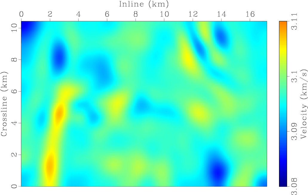
We have applied automatic migration velocity extraction by double path summation approach to the dataset.
Extracted velocity
distribution is shown in Figure 8. The velocity limits used for path-summation
integration correspond to
![]() and
and
![]() . They were chosen based on an
a priori migration velocity distribution.
. They were chosen based on an
a priori migration velocity distribution.
We used automatically extracted velocity to migrate initial (Figure 6)
and diffraction data (Figure 7). Images shown in the
Figures 6 and 7 are extracted from the whole migrated volume
along the target horizon - interface between coal layer and tight gas sand.
Diffraction image (Figure 7)
appears to have a high spatial resolution. It should be noticed that some of the most visible features
in the diffraction image can be identified in the conventional image as well.
For instance, the elliptical structure limited by inlines
![]() and crosslines
and crosslines
![]() is prominent in both images, but is more emphasized in the diffraction image. This observation
correlates with the fact that diffractions and reflections coexist on conventional images, but reflections
exhibit higher energy and may mask smaller-scale scatterers.
is prominent in both images, but is more emphasized in the diffraction image. This observation
correlates with the fact that diffractions and reflections coexist on conventional images, but reflections
exhibit higher energy and may mask smaller-scale scatterers.
We also performed unweighted
path-summation migration.
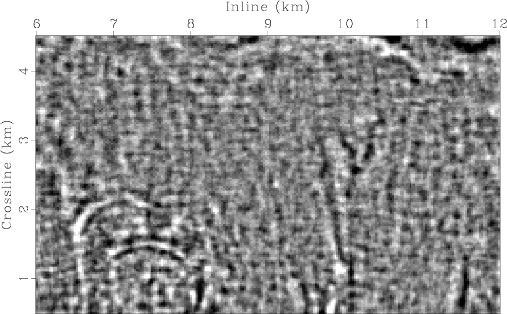
To illustrate the differences between the images
we focus on the area of the image corresponding to
![]() inlines and
inlines and
![]() crosslines.
Unweighted path-summation image (Figure 9c) has lower spatial resolution in comparison
to double path-summation velocity image (Figure 9a). However, the latter one appears to be noisier.
crosslines.
Unweighted path-summation image (Figure 9c) has lower spatial resolution in comparison
to double path-summation velocity image (Figure 9a). However, the latter one appears to be noisier.
A number of features such
as small faults corresponding to
![]() inlines and
inlines and ![]() crosslines and the elliptical structure
in the lower left corner of the figures look more focused on the double-path-summation image (Figure 9a) than
on the Figure 9e. This observation can be attributed
to double-path-summation migration velocity extraction directly from diffractions as opposed to PSTM velocity, which
has been estimated on
conventional full-waveform data containing significantly stronger reflections masking diffractions.
crosslines and the elliptical structure
in the lower left corner of the figures look more focused on the double-path-summation image (Figure 9a) than
on the Figure 9e. This observation can be attributed
to double-path-summation migration velocity extraction directly from diffractions as opposed to PSTM velocity, which
has been estimated on
conventional full-waveform data containing significantly stronger reflections masking diffractions.
Figure 9b shows an image acquired with double-path-summation migration velocity and a wider integration
range -
![]() . The image appears to be much less focused, however the pattern of the elliptical
structure can still be identified. Unweighted
path-summation migration image (Figure 9d)
appears to be significantly blurred due to overlap between tails and useful signal.
Gaussian weighting path-summation
scheme allows to significantly suppress tails and highlight actual apexes of hyperbolas (Figure 9f).
We used
. The image appears to be much less focused, however the pattern of the elliptical
structure can still be identified. Unweighted
path-summation migration image (Figure 9d)
appears to be significantly blurred due to overlap between tails and useful signal.
Gaussian weighting path-summation
scheme allows to significantly suppress tails and highlight actual apexes of hyperbolas (Figure 9f).
We used
![]() velocity bias with
velocity bias with ![]() . In comparison to Figure 9c
Gaussian weighting path-summation image
has lower spatial resolution. This observation is connected with wider integration range used for Gaussian
weighting path-summation migration
in comparison to the image 9c acquired with
. In comparison to Figure 9c
Gaussian weighting path-summation image
has lower spatial resolution. This observation is connected with wider integration range used for Gaussian
weighting path-summation migration
in comparison to the image 9c acquired with
![]() velocity limits. When a
wider integration range is used, area around the apex, within which diffraction hyperbolas are stacked coherently,
becomes larger leading to the resolution loss.
velocity limits. When a
wider integration range is used, area around the apex, within which diffraction hyperbolas are stacked coherently,
becomes larger leading to the resolution loss.


|
|---|
|
stack-cube,dif-cube
Figure 6. (a) Stacked volume; (b) volume after plane-wave destruction: diffractions are emphasized. |
|
|

|
|---|
|
conv-image-ts
Figure 7. Conventional reflection image acquired using double path-summation velocity shown in the Figure 8. |
|
|

|
|---|
|
dpi-ts
Figure 8. Diffraction image acquired using double path-summation velocity shown in the Figure 8. |
|
|
|
|---|
|
vel-hts-sing
Figure 9. Migration velocity distribution acquired by smooth division of double path-summation integral by path-summation integral according to equation A-5. |
|
|


|
|---|
|
w-dpi-ts,w-dpi-wr-ts,w-pathint-ts,w-pi-wr-ts,w-snt-dpi-ts,w-gpi-wr-ts
Figure 10. Integration range |
|
|
|
|
|
|
Analytical path-summation imaging of seismic diffractions |