|
|
|
|
Random noise attenuation using local signal-and-noise orthogonalization |
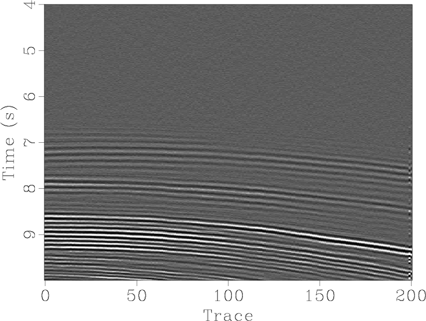
Figure 4a shows the unblended data for the first test, which is a deep-water common receiver section containing events that are nearly flat. After numerical blending using the same blending approach as in the first synthetic example, the blended data (shown in Figure 4c) demonstrate strong interference. Figure 4d shows the deblended data after the use of ![]() -
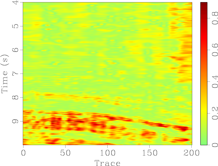
-![]() deconvolution. When checking the noise section in Figure 4e, we found many coherent signals, suggesting a significant leakage of useful signal energy. The denoised section after using the proposed approach is shown in Figure 4g. The noise section no longer contains coherent useful signals while the removed blending noise appears nearly unchanged. In this example, we set the vertical and lateral smoothing radii to 25 samples. The similarity maps before and after application of the proposed method are shown in Figure 4f and 4h. The SNR using the previous criteria of the blended data is 0.04. After the initial deblending using
deconvolution. When checking the noise section in Figure 4e, we found many coherent signals, suggesting a significant leakage of useful signal energy. The denoised section after using the proposed approach is shown in Figure 4g. The noise section no longer contains coherent useful signals while the removed blending noise appears nearly unchanged. In this example, we set the vertical and lateral smoothing radii to 25 samples. The similarity maps before and after application of the proposed method are shown in Figure 4f and 4h. The SNR using the previous criteria of the blended data is 0.04. After the initial deblending using ![]() -
-![]() deconvolution, SNR improves to 7.44. Further, after the proposed retrieving-signal process, SNR improves to 10.08. It is worth to be mentioned that the preservation of useful signal is of significant importance in deblending, and thus the proposed approach is particularly attractive in its application to deblending.
deconvolution, SNR improves to 7.44. Further, after the proposed retrieving-signal process, SNR improves to 10.08. It is worth to be mentioned that the preservation of useful signal is of significant importance in deblending, and thus the proposed approach is particularly attractive in its application to deblending.
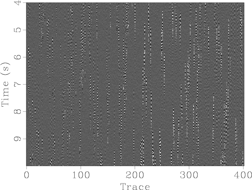
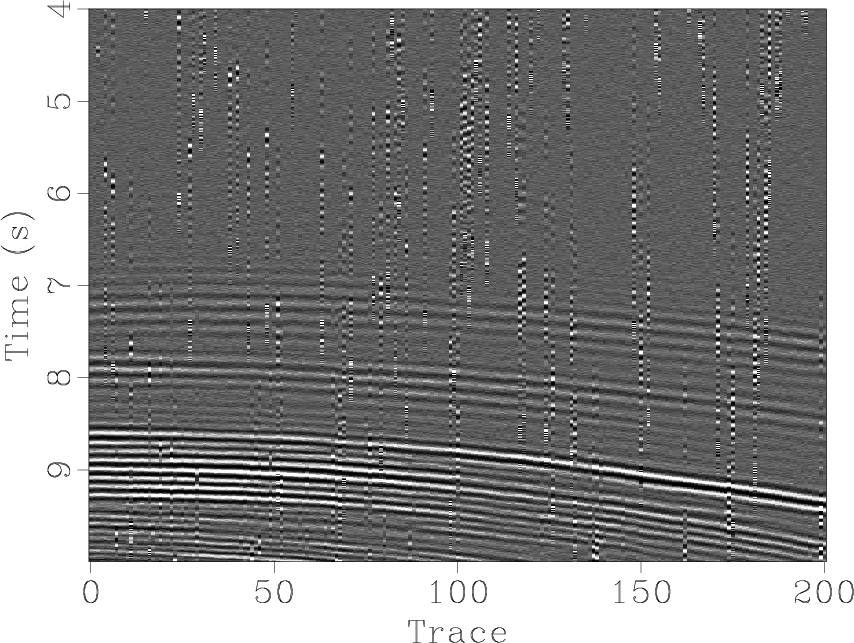
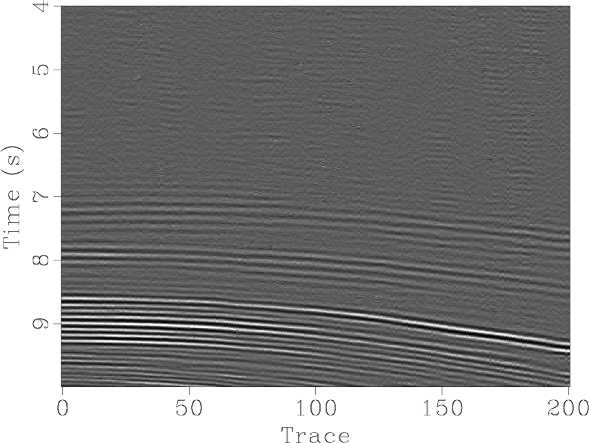
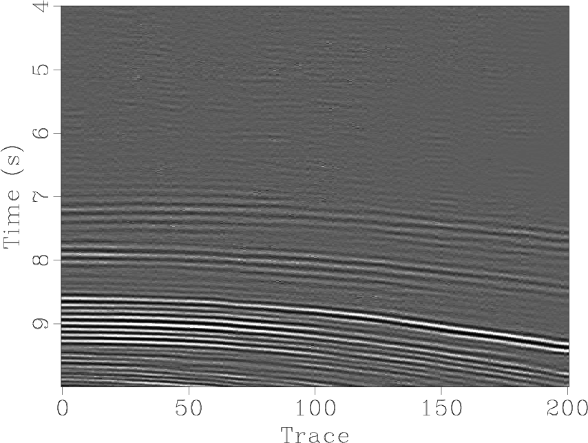
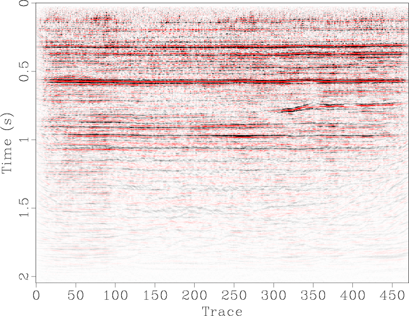
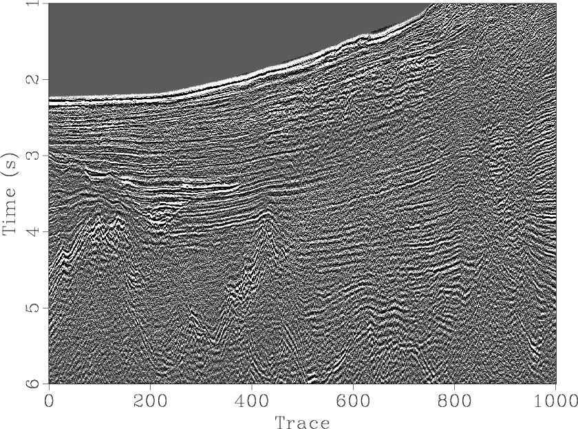
The second field data test is for a land seismic section, which was used previously by Fomel (2007a) and Liu and Fomel (2012). The input image is shown in Figure 5. The shallow part of the section is noisy, which may make interpretation difficult. After a conventional ![]() -
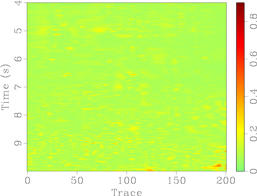
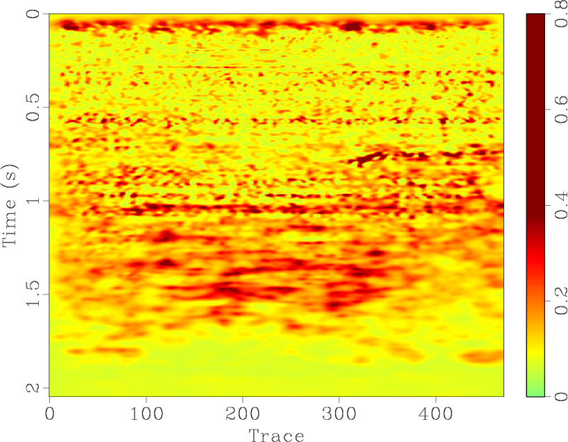
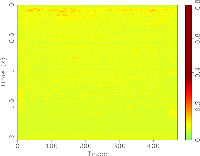
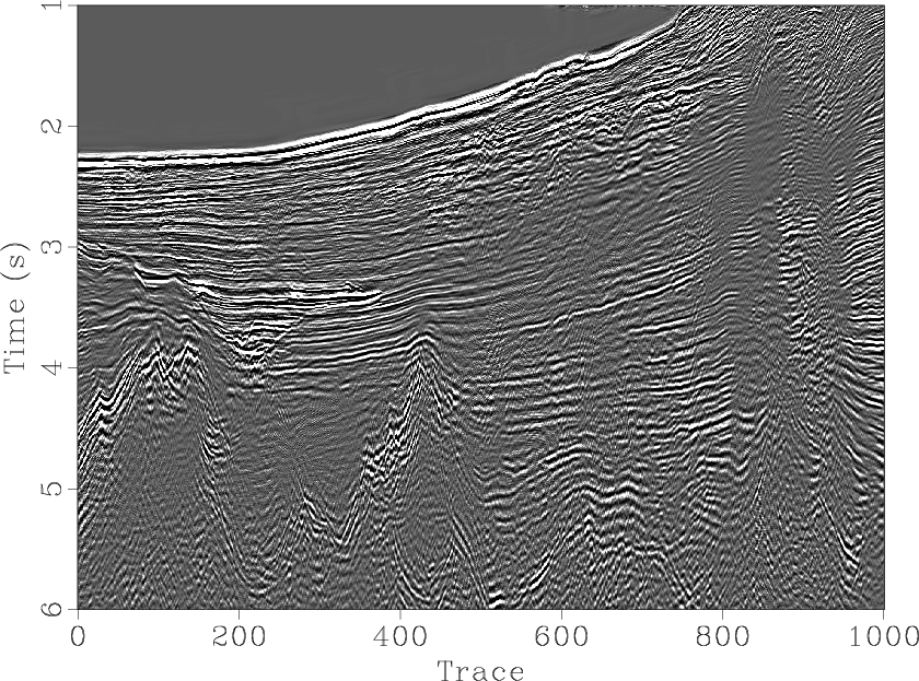
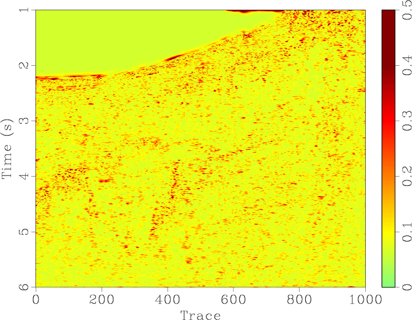
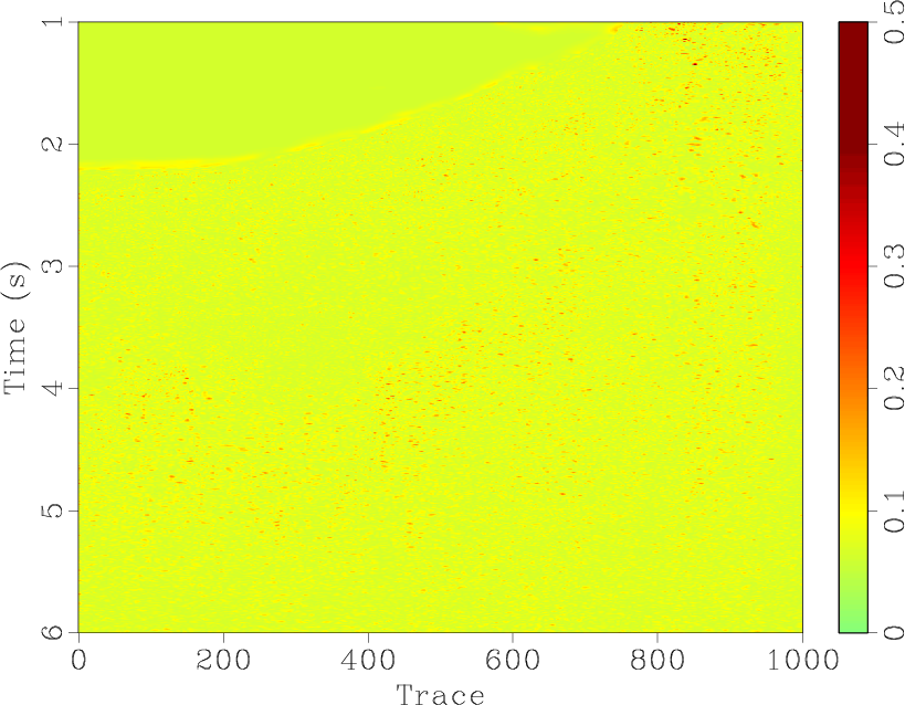
-![]() deconvolution, a much cleaner section is obtained (Figure 6a). Some coherent signal is left in the noise section shown in Figure 6d, especially around 0.75s and the 350th trace. After local signal-and-noise orthogonalization, we obtained a clean denoised section but with strong amplitude in some regions and almost no loss of useful component in the noise section (Figure 6d). In this example, the vertical and lateral smoothing radii are both 2 samples. Unlike the synthetic data test and the previous field data test, for this field data test, the clean signal is unknown, so the SNR measurement cannot be applied in this case. The two corresponding similarity maps are shown in Figure 7. The local similarity after applying the proposed approach is nearly zero along the whole seismic section.
deconvolution, a much cleaner section is obtained (Figure 6a). Some coherent signal is left in the noise section shown in Figure 6d, especially around 0.75s and the 350th trace. After local signal-and-noise orthogonalization, we obtained a clean denoised section but with strong amplitude in some regions and almost no loss of useful component in the noise section (Figure 6d). In this example, the vertical and lateral smoothing radii are both 2 samples. Unlike the synthetic data test and the previous field data test, for this field data test, the clean signal is unknown, so the SNR measurement cannot be applied in this case. The two corresponding similarity maps are shown in Figure 7. The local similarity after applying the proposed approach is nearly zero along the whole seismic section.


|
|---|
|
fairunblended2,fair-noise,fairblended2,fairdeblended2fx2,fairdeblended2dif-fx2,fairdif-simi,fairdeblended-ortho,fairdeblendeddif-ortho,fair-simi-ortho
Figure 4. Comparison of using the local-orthogonalization-based random noise attenuation approach for deblending test before and after. (a) Unblended section (not clean, also containing random noise). (b) Blending noise section. (c) Blended section. (d) Deblended result using |
|
|
|
|---|
|
pp
Figure 5. Noisy post-stack land field data (Fomel, 2013). |
|
|
|
|---|
|
pp-fx,pp-ortho,ppdiff-fx0,ppdiff-ortho0
Figure 6. (a) Denoised section using |
|
|
|
|---|
|
pp-simi,pp-simi-ortho
Figure 7. Comparison of similarity between noise section and denoised section with and without using the proposed random noise attenuation approach. (a) Similarity map using |
|
|
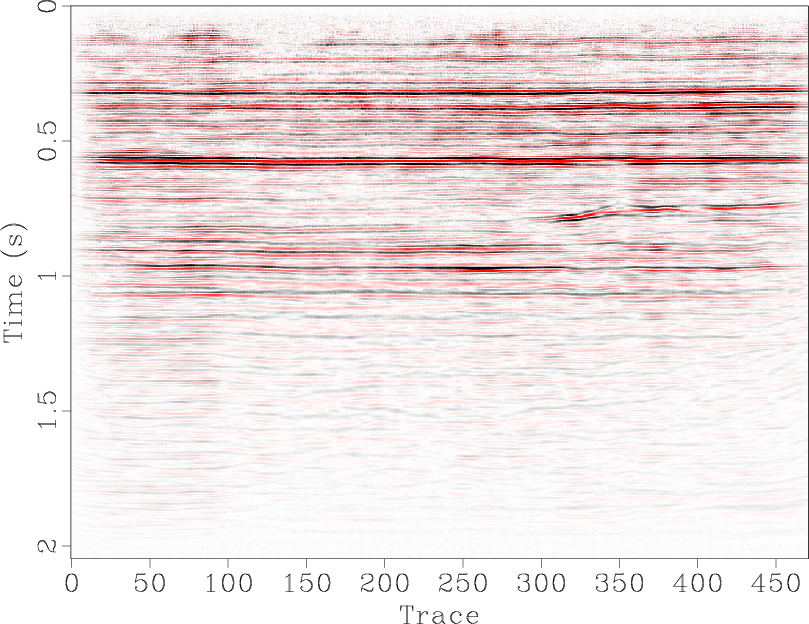
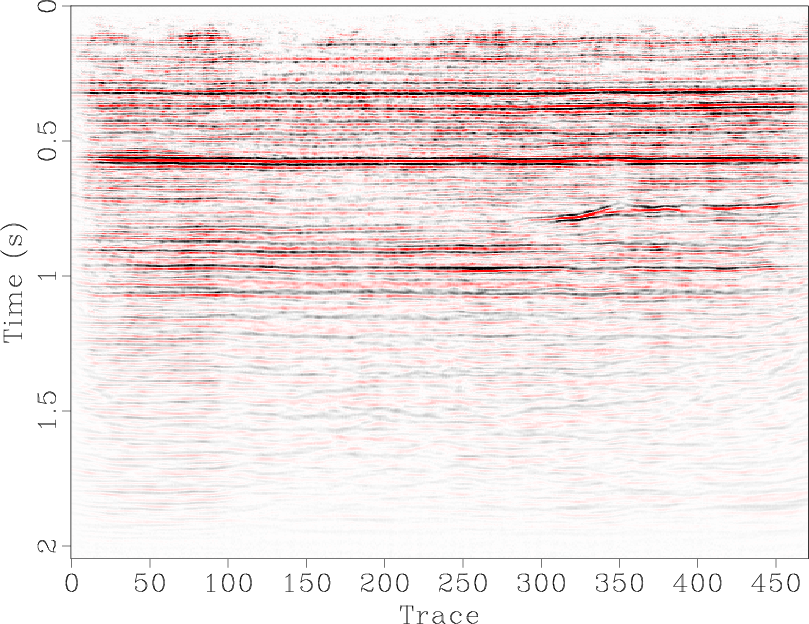
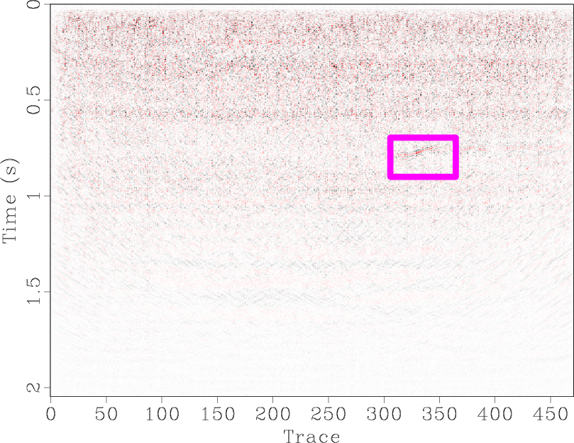
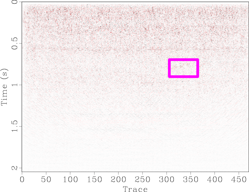
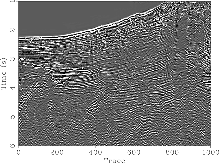
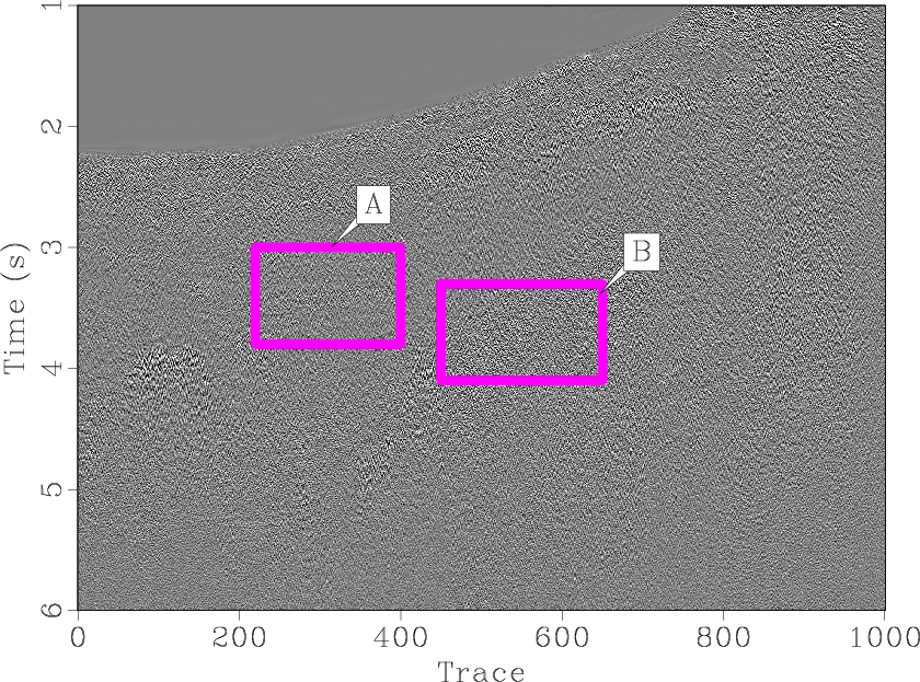
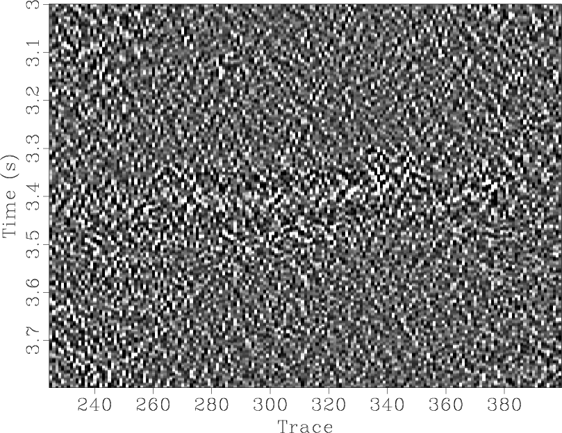
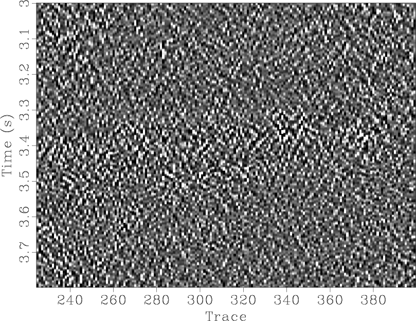
The third field data example is borrowed from Liu et al. (2012). The noisy data is shown in Figure 8. The initial signal and noise models are prepared using ![]() regularized nonstationary autoregression (RNAR). Following the approach of Liu et al. (2012), the initially denoised data are shown in Figure 9a. The corresponding noise section is shown in Figure 9c. The general denoising approach shows good performance considering the clean denoised image and random removed noise. However, we can find small useful signals from the noise section, as indicated by the frame boxes in Figure 9c. The denosied image using the proposed approach is shown in Figure 9b. After using local orthogonalization to retrieve useful signal, the coherent signal disappears in the final noise section (Figure 9d), as indicated by the frame boxes. The zoomed sections corresponding to frame boxes A and B in Figure 9 are shown in Figure 10. In this example, we chose the vertical and lateral smoothing radius as 5 samples. Before using the proposed approach, the local similarity map between the denoised data and removed noise (Figure 11a) showed some high-similarity anomalies. After applying the proposed approach, the similarity map is nearly zero everywhere across the whole section.
regularized nonstationary autoregression (RNAR). Following the approach of Liu et al. (2012), the initially denoised data are shown in Figure 9a. The corresponding noise section is shown in Figure 9c. The general denoising approach shows good performance considering the clean denoised image and random removed noise. However, we can find small useful signals from the noise section, as indicated by the frame boxes in Figure 9c. The denosied image using the proposed approach is shown in Figure 9b. After using local orthogonalization to retrieve useful signal, the coherent signal disappears in the final noise section (Figure 9d), as indicated by the frame boxes. The zoomed sections corresponding to frame boxes A and B in Figure 9 are shown in Figure 10. In this example, we chose the vertical and lateral smoothing radius as 5 samples. Before using the proposed approach, the local similarity map between the denoised data and removed noise (Figure 11a) showed some high-similarity anomalies. After applying the proposed approach, the similarity map is nearly zero everywhere across the whole section.
|
|---|
|
data
Figure 8. Noisy post-stack field data (Liu et al., 2012). |
|
|

|
|---|
|
npre,rna-ortho,nprediff0,rnadiff-ortho0
Figure 9. (a) Denoised section using |
|
|

|
|---|
|
zoom-rnadif-a,zoom-orthodif-a,zoom-rnadif-b,zoom-orthodif-b
Figure 10. (a) Zoomed section using |
|
|
|
|---|
|
rna-simi,rna-simi-ortho
Figure 11. Comparison of similarity between noise section and denoised section with and without using the proposed random noise attenuation approach. (a) Similarity map using |
|
|
|
|
|
|
Random noise attenuation using local signal-and-noise orthogonalization |