|
|
|
|
Omnidirectional plane-wave destruction |

|
|---|
|
lidl20,lidl50,lidl80,oidl20,oidl50,oidl80
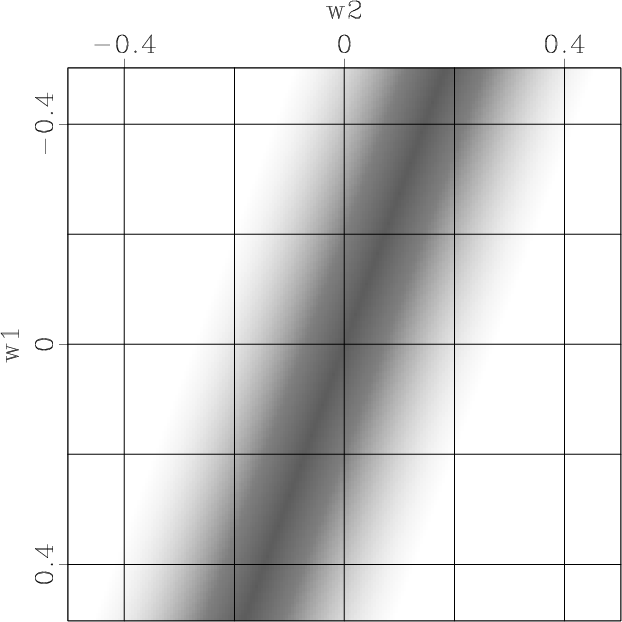
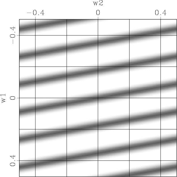
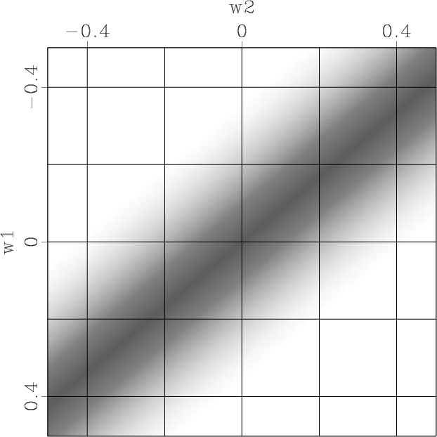
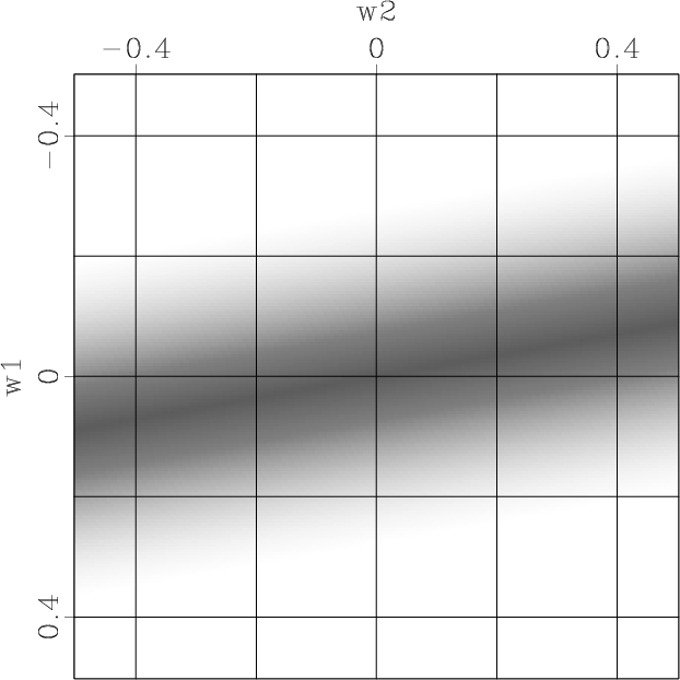
Figure 2. Magnitude responses of the line-interpolating PWD |
|
|
We compare the line-interpolating and circle-interpolating PWD operators
in the frequency domain.
At different dip angles,
the magnitude responses of
![]() and
and
![]() are shown in Figure 2:
When dip angle
are shown in Figure 2:
When dip angle
![]() , the two operators have similar responses
(Figure 2a and
2d);
when
, the two operators have similar responses
(Figure 2a and
2d);
when
![]() , the line-interpolating PWD become slightly aliased
(Figure 2b),
while the circle-interpolating PWD
is not aliased
(Figure 2e);
as
, the line-interpolating PWD become slightly aliased
(Figure 2b),
while the circle-interpolating PWD
is not aliased
(Figure 2e);
as ![]() increases to
increases to ![]() , the former is badly aliased
(Figure 2c),
and the latter is still not aliased
(Figure 2f).
, the former is badly aliased
(Figure 2c),
and the latter is still not aliased
(Figure 2f).
In summary, the line-interpolating PWD has different frequency responses for different dip angles. It may become aliased when the slope is large. The circle-interpolating PWD avoids aliasing for both small and large dip angles.
In line-interpolating PWD,
we must design a digital filter to approximate
the linear phase operator (or phase shift operator) ![]() .
The slope has an infinite range
.
The slope has an infinite range
![]() .
In circle-interpolating PWD,
there are two linear phase operators
.
In circle-interpolating PWD,
there are two linear phase operators ![]() and
and ![]() ,
related to the respective directions.
Both the slopes
,
related to the respective directions.
Both the slopes ![]() have a finite range
have a finite range ![]() .
.
Following Fomel (2002), the phase shift operators can be approximated by the following maxflat fractional delay filter (Thiran, 1971):
 |
(4) |
|
|---|
|
wrap
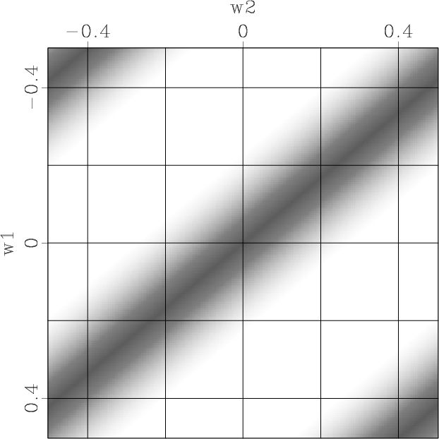
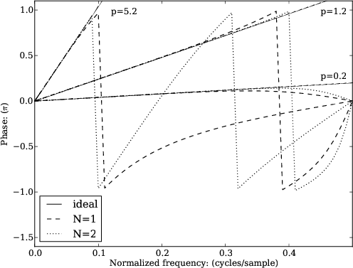
Figure 3. Phase approximating performances of the maxflat fractional delay filter |
|
|
In Figure 3, we show the phase approximating performances
of the maxflat fractional delay filters for different slopes. For
small slope ![]() , the approximations are good, but when the slopes
become large, the phases get wrapped. It is obvious
that the phase wrapping comes when and only when
, the approximations are good, but when the slopes
become large, the phases get wrapped. It is obvious
that the phase wrapping comes when and only when ![]() . The larger
the slope
. The larger
the slope ![]() , the more narrow
the linear-phase frequency bands become.
, the more narrow
the linear-phase frequency bands become.
As mentioned above, in line-interpolating PWC,
the slope ![]() is in the infinite interval
is in the infinite interval
![]() .
For steep structures,
where the slope
.
For steep structures,
where the slope ![]() becomes larger than
becomes larger than ![]() ,
there may be phase wrapping in the linear phase approximator.
However, in circle-interpolating PWC,
the ranges of
,
there may be phase wrapping in the linear phase approximator.
However, in circle-interpolating PWC,
the ranges of ![]() can be easily controlled by the radius
can be easily controlled by the radius ![]() .
If we choose
.
If we choose ![]() ,
the circle-interpolating can avoid phase wrapping completely for all dip angles.
,
the circle-interpolating can avoid phase wrapping completely for all dip angles.
|
|
|
|
Omnidirectional plane-wave destruction |