|
|
|
|
Omnidirectional plane-wave destruction |
Event picking is a useful tool for interpretation. However, when there are salt bodies and buried hills in our images, picking becomes difficult. Using some additional information, such as cross-correlation analysis (Yung and Ikelle, 1997), high-order statistics (Srinivasan and Ikelle, 2001) or local slope fields (Fomel, 2010), automatic picking tools can be improved. A challenge for automatic picking is therefore the robust estimation of the statistics or slope fields. This challenge is especially difficult near boundaries of salt bodies and buried hills because of steep structures. In this paper, we use the slope-based predictive painting method (Fomel, 2010) to pick events. We use the proposed OPWD to estimate the slope field, and show how it improves event-picking results.
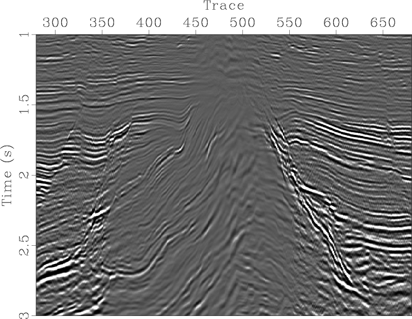
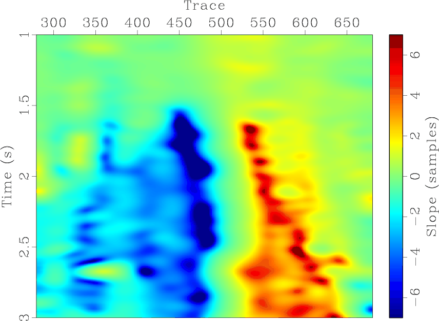
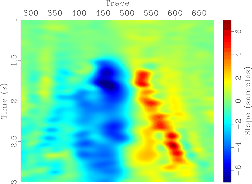
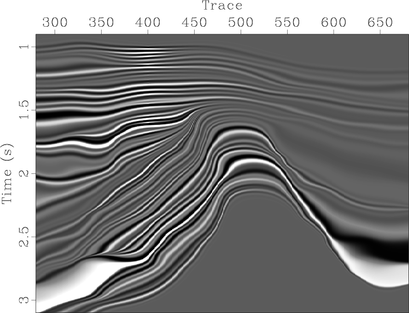
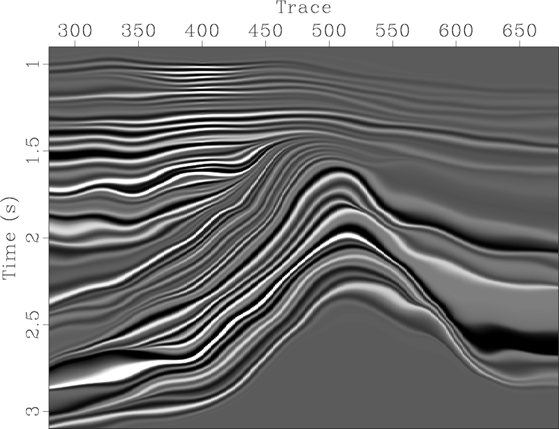
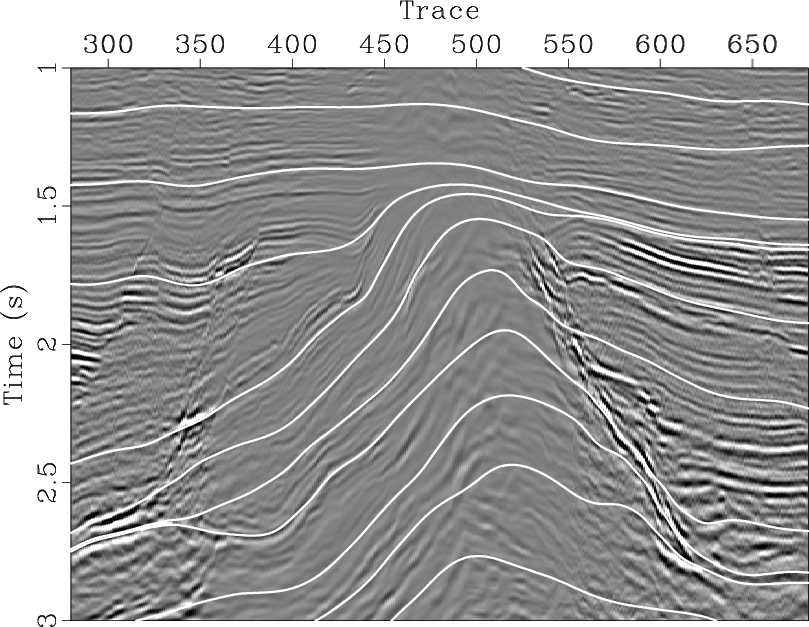
In Figure 7, we show a profile of a post-stack dataset from an oilfield in China. We can see a buried hill in this area, and there are several steep boundaries and faults near the buried hill. The slope field estimated by OPWD is shown in Figure 8a. Compared with the slope by LPWD in Figure 8b, the OPWD yields a larger estimated slope near the 360-th trace and the 475-th trace. As shown in Figure 7, there exist faults and steep buried-hill boundaries at these two positions, respectively. In this application, we use the shaping regularization with 25-points window size. We choose the 400-th and 560-th traces as two reference traces and use the two slope fields in 2D predictive painting. Painting results are shown in Figure 9a and Figure 9b. Meanwhile, we pick some of the events, as shown in Figure 10. Compared with the painting and picking results based on the LPWD, the OPWD provides more reasonable results near the fault (360-th trace) and near the buried-hill boundaries (475-th trace).
|
|---|
|
data
Figure 7. Field data example: steep structures and faults are rich in this selected area. |
|
|
|
|---|
|
odip,dip
Figure 8. Slope field estimated by OPWD (a) and LPWD (b). In both the two methods, we choose |
|
|
|
|---|
|
pred-odip,pred-dip
Figure 9. Predictive painting results using the OPWD slope (a) and LPWD slope (b): the reference traces are the 400-th and 560-th traces. |
|
|

|
|---|
|
pick-odip,pick-dip
Figure 10. Predictive picking results using the OPWD slope (a) and LPWD slope (b). |
|
|
|
|
|
|
Omnidirectional plane-wave destruction |