next up previous [pdf]

Next: Two-layer Model Up: Examples Previous: Examples

Complex-valued Lowrank Approximation

vel1d
Figure 1.
One-dimensional velocity profile with a sharp interface.
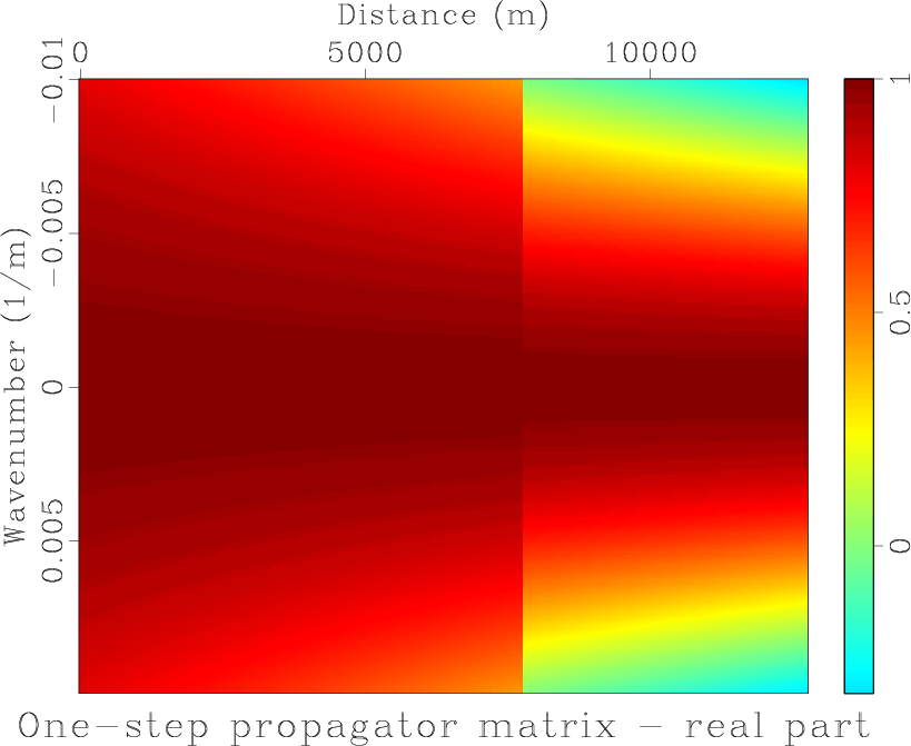
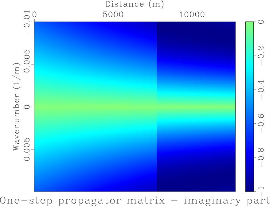
vel1d
[pdf] [png] [scons]

propr propi
propr,propi
Figure 2.
(a) The real part of the wave extrapolation matrix; (b) the imaginary part of wave extrapolation matrix.
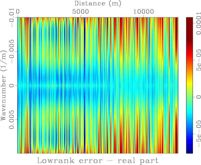
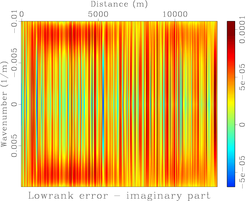
[pdf] [pdf] [png] [png] [scons]

proderr1r proderr1i
proderr1r,proderr1i
Figure 3.
(a) The real part of the approximation error; (b) the imaginary part of the approximation error.
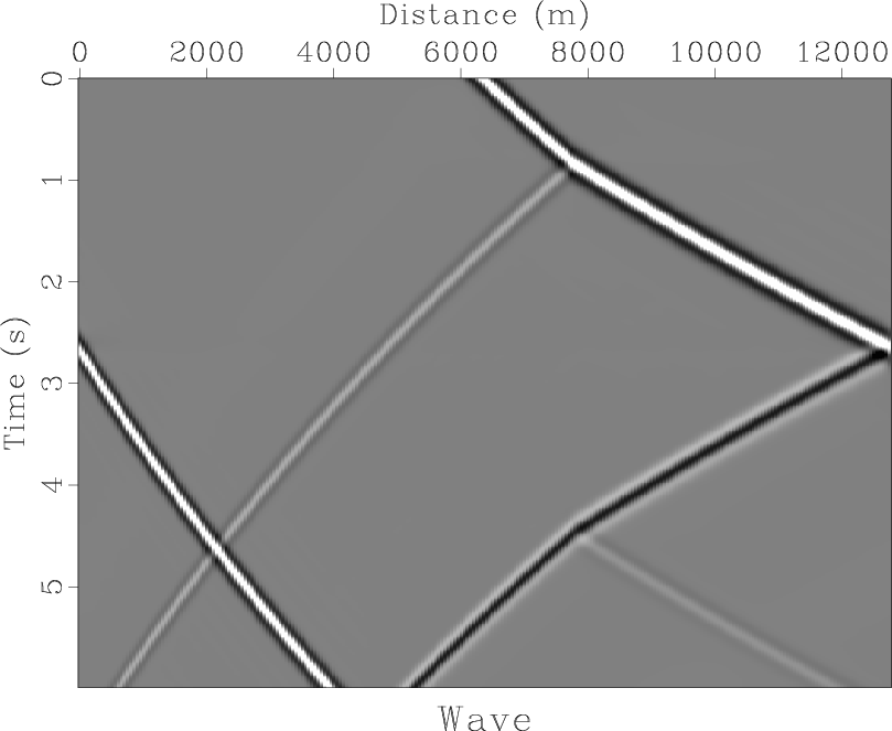
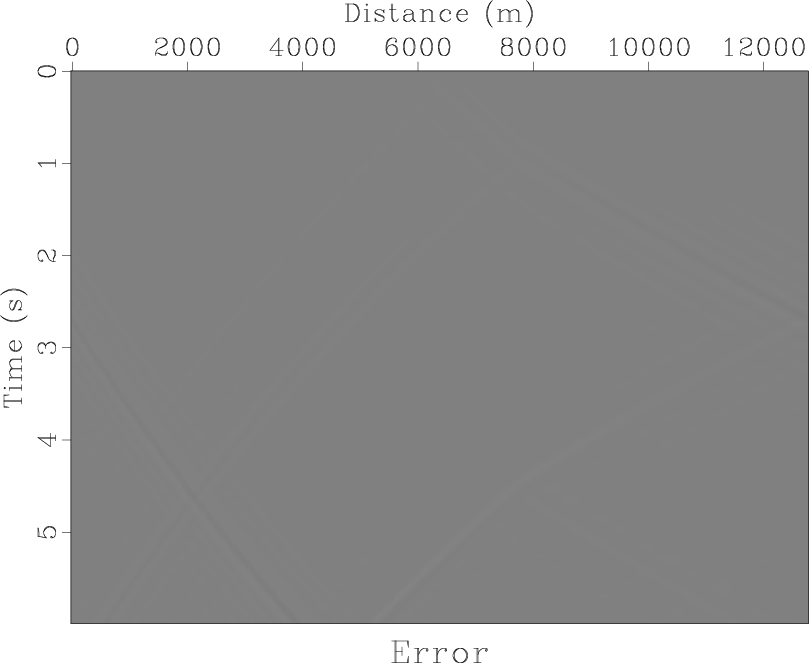
[pdf] [pdf] [png] [png] [scons]

wave2 error
wave2,error
Figure 4.
(a) 1D wave propagation from an initial condition - exact solution; (b) error of lowrank wave extrapolation.
[pdf] [pdf] [png] [png] [scons]

We first test the accuracy of lowrank approximation applied to wave extrapolation matrix in a 1D inhomogeneous medium. Using a simple velocity profile with a sharp velocity contrast (Figure 1), and a time step size of $ 0.01\;s$ , the real and imaginary part of the wave extrapolation matrix defined by Equation 25 with only the $ \phi_1$ term are plotted in Figures 2a and 2b, respectively. An accuracy threshold of $ \epsilon=10^{-4}$ leads to an approximation rank $ N=4$ . The approximation error is plotted in Figures 3a and 3b and shows the maximum error corresponding to the prescribed accuracy requirement. To see that the accuracy threshold is strick enough to guarantee kinematic accuracy, we first use an exact matrix multiplication to calculate the exact wavefield from an initial condition (Figure 4a). Next, we use lowrank wave extrapolation to compute the wavefield and calculate their difference (Figure 4b). Negligible error can be observed from the difference section, indicating the high accuracy of lowrank wave extrapolation.


next up previous [pdf]

Next: Two-layer Model Up: Examples Previous: Examples

2016-11-16