We proposed to compute the time-frequency map of an input signal based on
NPM coupled with Hilbert spectral analysis.
The proposed method is an empirical mode decomposition-like method, but using NPM
to compute its intrinsic mode functions. Compared with the Fourier
transform, the proposed method is data-driven and needs much less base functions
to approximate the original signal. Since the NPM
results an under-determined linear system, we use shaping regularization to
regularize it. The regularization makes the intrinsic mode functions more
smooth with respect to the amplitudes and frequencies
compared with the intrinsic mode functions of the empirical mode decomposition.
There are many time-frequency methods, which one is the best? This is a difficult
question to answer. Methods are good for some type signals, maybe not good for
other type signals.
Yung-Huang et al. (2014) pointed out that the complexity of empirical mode decomposition/ensemble
empirical mode decomposition is
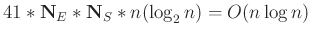 , where
  is the data length and the parameters
 and
and
 are the
ensemble and sifting numbers respectively. For the non-stationary Prony method, the computation
complexity is mainly attributed to the polynomial zero-finding. We used the pseudo-zeros
method to compute the pseudo-spectra of the associated balanced
companion matrix (Toh and Trefethen, 1994), which requires approximate
are the
ensemble and sifting numbers respectively. For the non-stationary Prony method, the computation
complexity is mainly attributed to the polynomial zero-finding. We used the pseudo-zeros
method to compute the pseudo-spectra of the associated balanced
companion matrix (Toh and Trefethen, 1994), which requires approximate
 works, where
 is the polynomial degree number. Therefore, the total computation complexity is
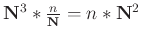 , where is the data length.
In this paper, we choose
, where is the data length.
In this paper, we choose
 , and therefore the total computation complexity is approximate
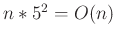 .
.
2020-07-18