|
|
|
|
Data-driven time-frequency analysis of seismic data using non-stationary Prony method |
Next: Appendix B: non-stationary Prony Up: Data-driven time-frequency analysis of Previous: ACKNOWLEDGMENTS
|
|
|
|
Data-driven time-frequency analysis of seismic data using non-stationary Prony method |
|
|
|
|
Data-driven time-frequency analysis of seismic data using non-stationary Prony method |
![$\displaystyle x[n] \approx \sum_{k=1}^{M}A_k e^{(\alpha_k + j\omega_k)(n-1)\Delta t + j\phi_k},$](img57.png)
![$\displaystyle x[n] \approx \sum_{k=1}^{M}h_k z_k^{n-1}.$](img63.png)
![$\displaystyle \mathbf{min} \sum_{n=1}^{N} \left\vert\epsilon[n]\right\vert^2 =
...
...{min}\sum_{n=1}^{N}\left \vert x[n] - \sum_{k=1}^{M}h_k z_k^{n-1}\right\vert^2.$](img64.png)
![$\displaystyle x[n] = \sum_{k=1}^{M}h_k z_k^{n-1}.$](img15.png)
![$\displaystyle \left[ \begin{array}{cccc}
z_1^0 & z_2^0 & \cdots & z_M^0\\
z_1^...
...ht] =
\left[ \begin{array}{c} x[1] x[2] \vdots x[M]
\end{array} \right].$](img16.png)
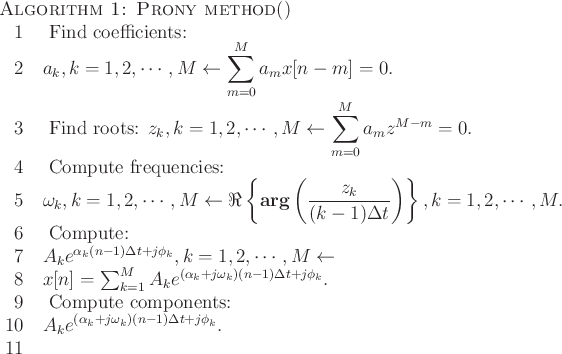
![$\displaystyle \sum_{m=0}^{M}a_mx[n-m] = \sum_{k=1}^{M}h_kz_k^{n-M-1}
\sum_{m=0}^M a[m]z_{k}^{M-m}.$](img68.png)
![$\displaystyle \sum_{m=0}^{M}a_mx[n-m] = 0.$](img21.png)