Seismic data decomposition into spectral components using regularized nonstationary autoregression

Examples

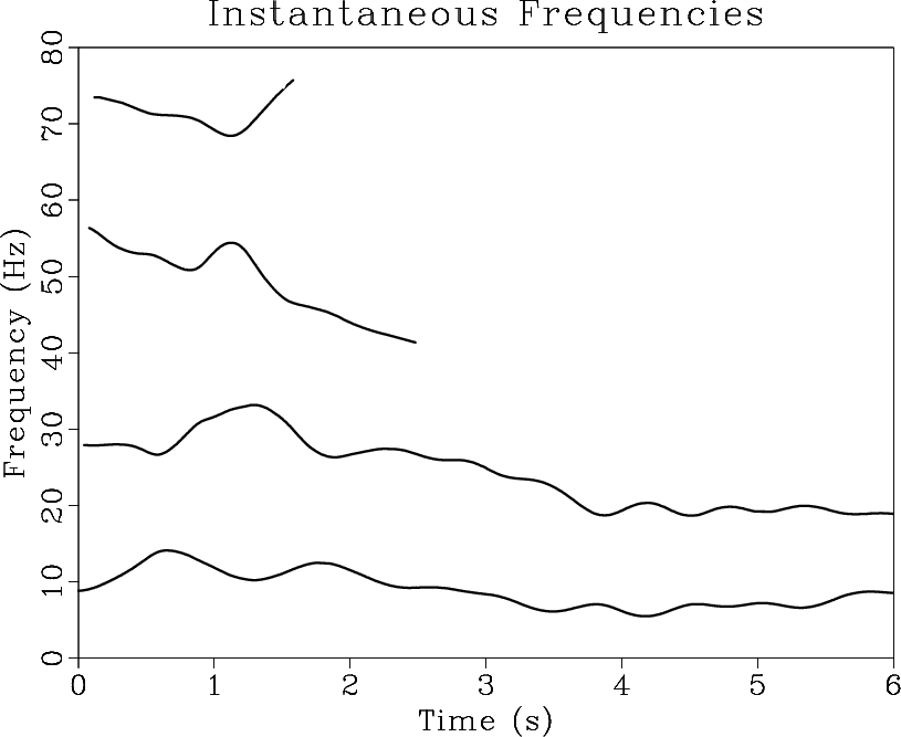
To illustrate performance of the proposed approach in field-data applications, I first use a simple 1D example: a single seismic trace from a marine survey. Figure 10 shows the input trace and the output of RNAR, with a five-point adaptive prediction-error filter. The four variable instantaneous frequencies extracted from the roots of the filter are shown in Figure 11. They correspond to four different spectral components extracted from the data in Step 3 (Figure 12.) Surprisingly, only four components with smoothly varying frequencies and amplitudes are sufficient to describe a significant portion of the signal, including the effect of attenuating frequencies at later times (Figure 13.)

cerr
Figure 10. Seismic trace and residual after adaptive prediction-error filtering with RNAR.

tgroup
Figure 11. Instantaneous frequencies of four components extracted from seismic trace in Figure 10 using RNAR.

csign
Figure 12. Four nonstationary spectral components corresponding to frequencies in Figure 11.

cfit
Figure 13. Fitting input seismic trace with sum of four spectral components shown in Figure 12.

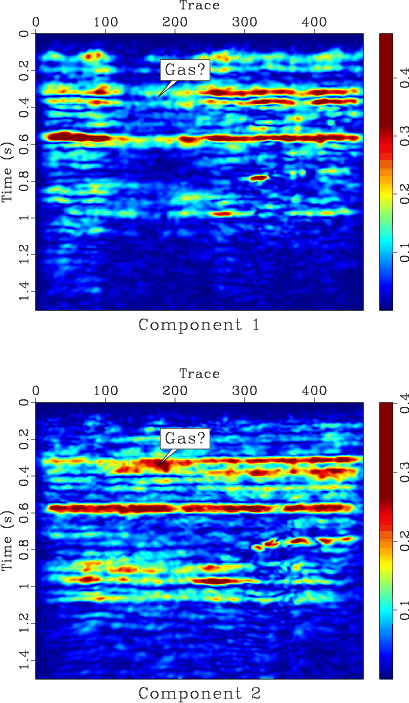
The second example is a 2D section from a land seismic survey (Figure 14a), analyzed previously by Fomel (2007) and Liu and Fomel (2013). I choose a three-point prediction-error filter to highlight the two most significant data components. The fitting error is shown in Figure 15 and contains mostly random noise. The two estimated spectral components are shown in Figure 16, with the corresponding instantaneous frequencies $f_n)t)$ shown in Figure 17. The corresponding amplitudes $\vert\hat{A}_n(t)\vert$ are shown in Figure 18. Comparing frequency and amplitude attributes from different components, a low-frequency anomaly (a zone of attenuated high frequencies) in the top-left part of the section becomes apparent. This anomaly might indicate presence of gas (Castagna et al., 2003).

vdata
Figure 14. (a) 2D seismic data section. (b) Result of fitting data with two components shown in Figure 16.

vdif
Figure 15. Residual error after fitting seismic data from Figure 14 with two components shown in Figure 16.

vsign
Figure 16. Two nonstationary spectral components: high-frequency (Component 1) and low-frequency (Component 2) estimated from the data shown in Figure 14a.

vgroup
Figure 17. Instantaneous frequencies of high-frequency and low-frequency components from decomposition shown in Figure 16.

vcwht
Figure 18. Amplitudes of high-frequency and low-frequency components from decomposition shown in Figure 16. The apparent attenuation of high frequencies in the top left part of the section may indicate presence of gas.

Seismic data decomposition into spectral components using regularized nonstationary autoregression