Seismic data decomposition into spectral components using regularized nonstationary autoregression

Autoregressive spectral analysis

Prony's method of data analysis was developed originally for representing a noiseless signal as a sum of exponential components (Prony, 1795). It was extended later to noisy signals, complex exponentials, and spectral analysis (Pisarenko, 1973; Beylkin and Monzón, 2005; Marple, 1987; Bath, 1995). The basic idea follows from the fundamental property of exponential functions: $e^{\alpha\,(t+\Delta t)} = e^{\alpha\,t}\,e^{\alpha\,\Delta t}$. In signal-processing terms, it implies that a time sequence $d(t)=A\,e^{\alpha\,t}$ (with real or complex $\alpha$) is predictable by a two-point prediction-error filter $\left(1,-e^{\alpha\,\Delta t}\right)$, or, in the Z-transform notation,

$$F_0(Z) = 1-Z/Z_0\;,$$ (6)

where $Z_0 = e^{-\alpha\,\Delta t}$. If the signal is composed of multiple exponentials,

$$d(t) \approx \sum\limits_{n=1}^{N} A_n\,e^{\alpha_n\,t}\;,$$ (7)

they can be predicted simultaneously by using a convolution of several two-point prediction-error filters:

$$F(Z) = (1-Z/Z_1)\, (1-Z/Z_2)\,\cdots\, (1-Z/Z_N)$$

$$= 1 + a_1\,Z + a_2\,Z^2 + \cdots + a_n\,Z^N\;,$$ (8)

where $Z_n = e^{-\alpha_n\,\Delta t}$. This observation suggests the following three-step algorithm:

1. Estimate a prediction-error filter from the data by determining filter coefficients $a_1, a_2, \ldots, a_N$ from the least-squares minimization of
   

   $$e(t) = d(t) - \sum_{n=1}^{N} a_n\,d(t-n\,\Delta t)\;.$$ (9)

   
   

2. Writing the filter as a $Z$ polynomial (equation 8), find its complex roots $Z_1, Z_2, \ldots, Z_N$. The exponential factors $\alpha_1, \alpha_2, \ldots, \alpha_N$ are determined then as
   

   $$\alpha_n = -\ln(Z_n)/\Delta t\;.$$ (10)

   
   

3. Estimate amplitudes $A_1,A_2, \ldots, A_N$ of different components in equation 7 by linear least-squares fitting.

Prony's method can be applied in sliding windows, which was a technique developed by Russian geophysicists (Mitrofanov and Priimenko, 2011; Gritsenko et al., 2001) for identifying low-frequency seismic anomalies (Mitrofanov et al., 1998). I propose to extend it to smoothly nonstationary analysis by applying the following modifications:

1. Using RNAR, the filter coefficients $a_n$ become smoothly-varying functions of time $\hat{a}_n(t)$, which allows the filter to adapt to nonstationary changes in the input data.
2. At each instance of time, roots of the corresponding $Z$ polynomial also become functions of time $\hat{Z}_n(t)$. I apply a robust, eigenvalue-based algorithm for root finding (Toh and Trefethen, 1994). The instantaneous frequency of different components $f_n(t)$ is determined directly from the phase of different roots:
   

   $$f_n(t) = -Re\left[\arg\left(\frac{\hat{Z}_n(t)}{2\pi\,\Delta t}\right)\right]\;.$$ (11)

   
   

3. Finally, using RNR, I estimate smoothly-varying amplitudes of different components $\hat{A}_n(t)$.

The nonstationary decomposition model for a complex signal $d(t)$ is thus

$$d(t) \approx \sum\limits_{n=1}^{N} d_n(t)\;,\quad\mbox{where}\quad d_n(t) = \hat{A}_n(t)\,e^{i\,\phi_n(t)}$$ (12)

and the local phase $\phi_n(t)$ corresponds to time integration of the instantaneous frequency determined in Step 2:

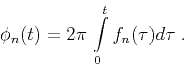$$\phi_n(t) = 2\pi\,\int\limits_{0}^{t} f_n(\tau) d\tau\;.$$ (13)

For ease of analysis, real signals can be transformed to the complex domain by using analytical traces (Taner et al., 1979).

Seismic data decomposition into spectral components using regularized nonstationary autoregression