|
|
|
|
Matching and merging high-resolution and legacy seismic images |
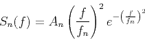
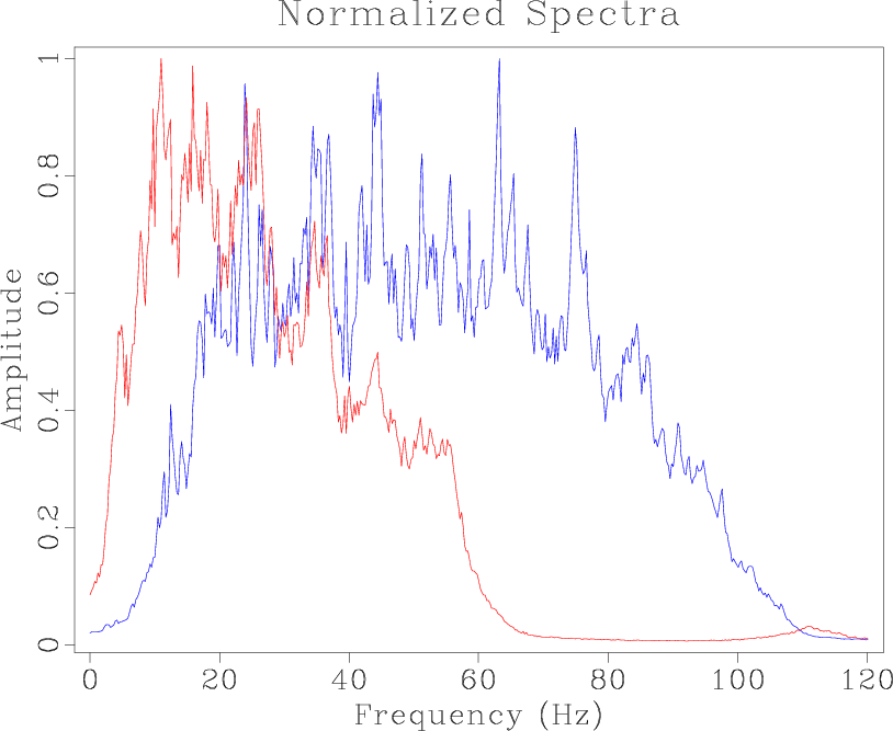
Analyzing the spectra of the legacy and high-resolution images, as seen in Figure 2a, it is clear that the high-resolution image has a wider range of frequencies with a higher dominant frequency than the legacy image. In order to match these images, our first step is to balance their spectral content. We can achieve this by attenuating the high frequencies of the high-resolution image to match the lower frequency content of the legacy image. One approach to frequency balancing is to apply a stationary bandpass filter to the high-resolution image. However, this does not take into account local frequency variations in each image caused by seismic wave attenuation. A more effective method, which accounts for temporally and spatially variable frequency content that is present in most seismic data, is to apply a non-stationary filter using frequency information from both images. To accomplish this, we use a simple triangle smoothing operator with an adjustable radius. Here, the radius at each point is the number of seconds that that specific data point gets averaged over in a triangle weight in the temporal direction. We specifically look at local frequency (Fomel, 2007), which is a time-dependent frequency attribute, and can be thought of as a smoothed estimate of instantaneous frequency (White, 1991). For the procedure described in this paper, local frequency is a better-suited attribute than instantaneous frequency. Local frequency allows the comparison of frequency content in a local region of samples, as opposed to instantaneous frequency, which allows for a point by point comparison of frequency values between images. Since the corresponding reflections between images may not be precisely aligned in time at this stage in the method, using the local frequency attribute to balance frequency content between images would allow for more accurate frequency balancing than instantaneous frequency.
|
|---|
|
nspectra,hires-smooth-spec
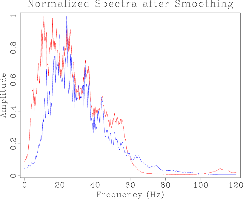
Figure 2. Spectra for the entire image display of the legacy (red) and high-resolution (blue) images before (a) and after (b) spectral balancing. |
|
|
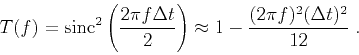
The justification for triangle smoothing is that it is a simple approximation to Gaussian smoothing. The frequency response of the triangle smoothing filter (Claerbout, 1992) is
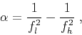
Because we are smoothing the high-resolution image to match it with the legacy image, we can relate the high-resolution frequencies, ![]() , to the legacy frequencies,
, to the legacy frequencies, ![]() , such that
, such that
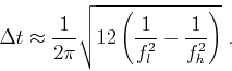
Combining equations (1), (2), and (5) leads to the specification of the triangle smoothing radius as
|
|---|
|
rect
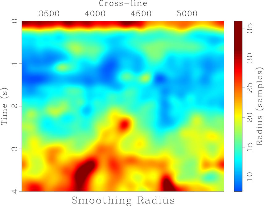
Figure 3. Calculated spatially and temporally variable smoothing radius. This represents the number of seconds in the temporal direction that the high-resolution image gets averaged over in a triangle weight to balance local frequency content with the legacy image at each sample. |
|
|
We measure local frequencies in both images and apply smoothing specified by equation (6) to the high-resolution image.
Since this is only an approximation of what the smoothing radius should be under ideal conditions, we adjust the constant ![]() in the equation to achieve a better match.
In this example, this effectively reduces the difference between the spectral content of the images, as shown in Figure 2b.
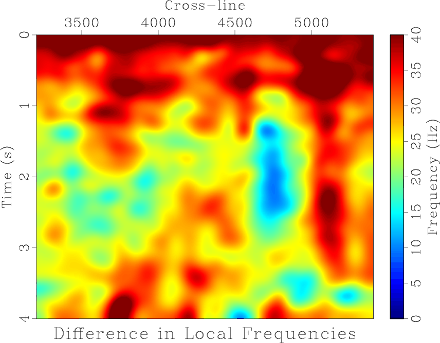
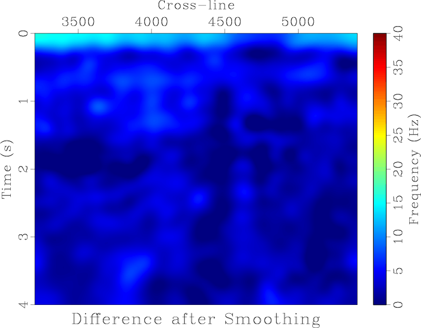
Figure 4 shows the difference in local frequencies before and after smoothing. After smoothing, the frequency difference is minimized.
in the equation to achieve a better match.
In this example, this effectively reduces the difference between the spectral content of the images, as shown in Figure 2b.
Figure 4 shows the difference in local frequencies before and after smoothing. After smoothing, the frequency difference is minimized.
This method works well for simple data sets with overlapping frequency content. However, more complicated data sets, as seen in the next example, may require additional steps for successful frequency balancing.
In addition to frequency balancing, we initially attempted accounting for wavelet phase differences between data sets at this step. However, we saw this had a negligible impact on the final result, so we decided not to include it in this method.
|
|---|
|
freqdif,freqdif-filt
Figure 4. Difference in local frequencies between the legacy and high-resolution images before (a) and after (b) balancing their frequency content by non-stationary smoothing. |
|
|
|
|
|
|
Matching and merging high-resolution and legacy seismic images |