Example II

Our second test is field data example from the Cranfield CO$_2$ sequestration experiment (Zhang et al., 2013). This dataset consists of baseline and monitor seismic images.

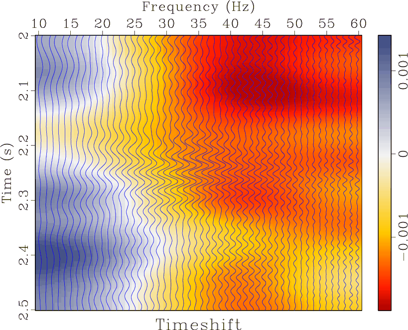
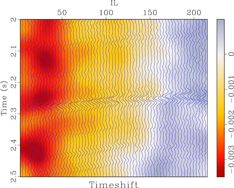
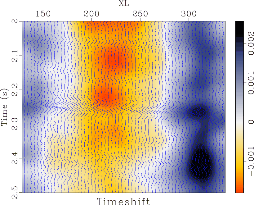
We follow the same workflow as described in the previous example. The time-lapse seismic images are decomposed into discrete frequency componenets using the local time frequency transform (Liu and Fomel, 2013) and timeshifts are estimated using amplitude-adjusted plane-wave destruction filters (Phillips and Fomel, 2016). To test the effectiveness of this algorithm, we interleave slices of the baseline and monitor images on top of the corresponding timeshift estimate map (Figure 4). The apparent “zig-zag" patterns between the traces indicate the images are not optimally aligned for time-lapse analysis. These patterns coincide with large timeshift estimates. Upon shifting the monitor image, the reflections are optimally aligned.

fdip,idip,xdip
Figure 4. Timeshift estimates as a function of (a) frequency, (b) inline, and (c) crossline. Overlying traces are interleaved baseline and monitor images. Areas with large timeshift (bright color) correspnd to misalignment between baseline and monitor images.

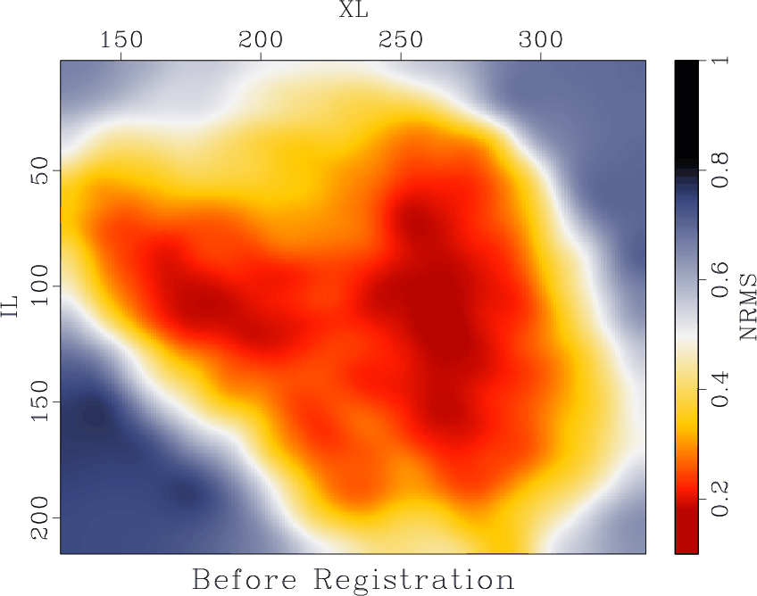
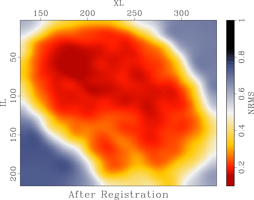
The normalized root-mean-square (NRMS) attribute is computed before and after shifting the monitor image (Figure 5). Lower NRMS values indicate coherent signal in the time-lapse residual corresponding to misalignment between the time-lapse seismic images has been eliminated.

nrms1,nrms2
Figure 5. NRMS maps (a) before and (b) after registration. Low NRMS values indicate that the application of estimated timeshifts effectively destroys most coherent signal in the time-lapse residual.