|
|
|
|
Estimation of timeshifts in time-lapse seismic images using spectral decomposition |
Next: Example I Up: Phillips and Fomel: Timeshifts Previous: Introduction
|
|
|
|
Estimation of timeshifts in time-lapse seismic images using spectral decomposition |
 -transform notation as
 |
(1) |
where  is a warping filter,
  is a phase shift between time-lapse seismic images,
  is an amplitude weight, and
  is the 4D timeshift.
This assumption fails when layers are below seismic resolution and significant interference between reflection sidelobes exists.
We partially alleviate the problem of interference by decomposing seismic images into discrete frequency components using the local time-frequency transform (Liu and Fomel, 2013).
is the 4D timeshift.
This assumption fails when layers are below seismic resolution and significant interference between reflection sidelobes exists.
We partially alleviate the problem of interference by decomposing seismic images into discrete frequency components using the local time-frequency transform (Liu and Fomel, 2013).
The local-time-frequency transform is based on the idea of non-stationary regression.
A digital signal  can be represented as Fourier series
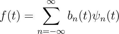 |
(2) |
where the Fourier coefficients  are allowed to vary temporally and
  is a vector consisting of complex exponentials at each corresponding Fourier frequency.
The Fourier coefficients
is a vector consisting of complex exponentials at each corresponding Fourier frequency.
The Fourier coefficients  are estimated by regularized least-squares inversion (Fomel, 2008).
We then use amplitude-adjusted plane-wave destruction filters (Phillips and Fomel, 2016) to estimate timeshifts at each frequency. In the linear operator notation, equation (1) is modified to
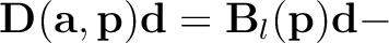 diag diag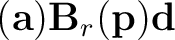 |
(3) |
where
 and
and
 are the left- and right-hand side of the plane-wave destruction filter (Fomel, 2002), as described by Phillips and Fomel (2016), and
 is the local time-frequency transform of the time-lapse seismic data.
Our objective is to minimize the plane-wave residual between the time-lapse seismic images at each frequency (
is the local time-frequency transform of the time-lapse seismic data.
Our objective is to minimize the plane-wave residual between the time-lapse seismic images at each frequency (
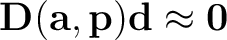 ).
).
The dependence of
 on
on
 is linear; however,
 enters in a non-linear way (Fomel, 2002).
We separate this problem into linear and non-linear parts using the variable projection technique (Golub and Pereyra, 1973; Kaufman, 1975).
The algorithm is described below (Phillips and Fomel, 2016):
enters in a non-linear way (Fomel, 2002).
We separate this problem into linear and non-linear parts using the variable projection technique (Golub and Pereyra, 1973; Kaufman, 1975).
The algorithm is described below (Phillips and Fomel, 2016):
 and
and
 .
constant and compute the shift
.
constant and compute the shift
 using accelerated plane-wave destruction (Chen et al., 2013).
constant and compute the amplitude ratio
using accelerated plane-wave destruction (Chen et al., 2013).
constant and compute the amplitude ratio
 by the smooth division of the left and right side of the plane-wave destruction filter
in equation(3):
by the smooth division of the left and right side of the plane-wave destruction filter
in equation(3):
 |
(4) |
If timeshifts are large (
 10 samples), rather than setting
, it may be necessary to instead provide a low frequency estimate of the timeshift calculated using another algorithm, such as local similarity (Fomel and Jin, 2009).
So long as this “small timeshift" condition is satisfied, this algorithm provides an improved estimate of true 4D timeshifts from spectrally decomposed time-lapse seismic images.
10 samples), rather than setting
, it may be necessary to instead provide a low frequency estimate of the timeshift calculated using another algorithm, such as local similarity (Fomel and Jin, 2009).
So long as this “small timeshift" condition is satisfied, this algorithm provides an improved estimate of true 4D timeshifts from spectrally decomposed time-lapse seismic images.
|
|
|
|
Estimation of timeshifts in time-lapse seismic images using spectral decomposition |