 |
 |
 |
 | Adaptive multiple subtraction using regularized nonstationary regression |  |
![[pdf]](icons/pdf.png) |
Next: Toy examples
Up: Stationary and nonstationary regression
Previous: Prediction-error filtering
Non-stationary regression uses a definition similar to
equation 1 but allows the coefficients  to change
with
to change
with  . The error turns into
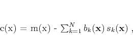 |
(2) |
and the problem of its minimization becomes ill-posed, because one can
get more unknown variables than constraints. The remedy is to include
additional constraints that limit the allowed variability of the
estimated coefficients.
The classic regularization method is Tikhonov's regularization
(Tikhonov, 1963; Engl et al., 1996), which amounts to minimization of the following
functional:
![\begin{displaymath}
F[\mathbf{b}] = \Vert e(\mathbf{x})\Vert^2 +
\epsilon^2...
...k=1}^{N} \Vert\mathbf{D}\left[b_k(\mathbf{x})\right]\Vert^2\;,
\end{displaymath}](img23.png) |
(3) |
where  is the regularization operator (such as the
gradient or Laplacian filter) and
is the regularization operator (such as the
gradient or Laplacian filter) and  is a scalar
regularization parameter. If is a linear operator,
least-squares estimation reduces to linear inversion
is a scalar
regularization parameter. If is a linear operator,
least-squares estimation reduces to linear inversion
 |
(4) |
where
![$\mathbf{b} = \left[\begin{array}{cccc}b_1(\mathbf{x}) & b_2(\mathbf{x}) & \cdots & b_N(\mathbf{x})\end{array}\right]^T$](img27.png) ,
,
![$\mathbf{d} = \left[\begin{array}{cccc}s_1(\mathbf{x})\,m(\mathbf{x}) & s_2(\mat...
...})\,m(\mathbf{x}) & \cdots & s_N(\mathbf{x})\,m(\mathbf{x})\end{array}\right]^T$](img28.png) ,
and the elements of matrix
,
and the elements of matrix  are
are
 |
(5) |
Shaping regularization (Fomel, 2007b) formulates the problem
differently. Instead of specifying a penalty (roughening) operator
, one specifies a shaping (smoothing) operator  .
The regularized inversion takes the form
.
The regularized inversion takes the form
 |
(6) |
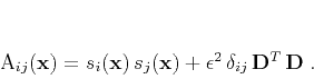
where
the elements of matrix
 are
are
![\begin{displaymath}
\widehat{A}_{ij}(\mathbf{x}) = \lambda^2\,\delta_{ij} +
...
...thbf{x})\,s_j(\mathbf{x}) -
\lambda^2\,\delta_{ij}\right]\;,
\end{displaymath}](img35.png) |
(7) |
and  is a scaling coefficient.The main advantage of this
approach is the relative ease of controlling the selection of
and in comparison with and
. In all examples of this paper, I define as
Gaussian smoothing with an adjustable radius and choose to
be the median value of
is a scaling coefficient.The main advantage of this
approach is the relative ease of controlling the selection of
and in comparison with and
. In all examples of this paper, I define as
Gaussian smoothing with an adjustable radius and choose to
be the median value of
 . As demonstrated in the next
section, matrix
is typically much better
conditioned than matrix , which leads to fast inversion
with iterative algorithms.
. As demonstrated in the next
section, matrix
is typically much better
conditioned than matrix , which leads to fast inversion
with iterative algorithms.
In the case of  (regularized division of two signals), a similar
construction was applied before to define local seismic
attributes (Fomel, 2007a).
(regularized division of two signals), a similar
construction was applied before to define local seismic
attributes (Fomel, 2007a).
|
|
|
|
| Adaptive multiple subtraction using regularized nonstationary regression | |
|
Next: Toy examples
Up: Stationary and nonstationary regression
Previous: Prediction-error filtering
2013-07-26