|
 |
 |
 | Theory of interval traveltime parameter estimation in layered anisotropic media |  |
![[pdf]](icons/pdf.png) |
Next: Comparison with the method
Up: Coefficients of traveltime expansion
Previous: Formulas for interval quartic
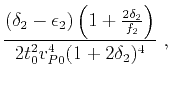
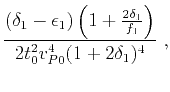
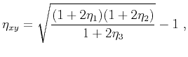
Al-Dajani et al. (1998) derived the following expressions for  and
and  :
:
where
 and
and
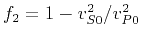 ,
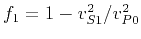
,  is the vertical qP-wave velocity,
  is the qS-wave velocity polarized in
![$ {[x_1,x_3]}$](img187.png) , and
, and  is the qS-wave velocity polarized in
![$ {[x_2,x_3]}$](img190.png) . The subscript in anisotropic parameters denotes the index of the normal direction to the associated plane. Note that equation 56 is similar to the VTI expression with corresponding changes in the anisotropic parameters for different planes. This result is due to the similarity of the Christoffel equations in the case of VTI media and in-symmetry-plane orthothombic media (Tsvankin, 2012). The expression for
. The subscript in anisotropic parameters denotes the index of the normal direction to the associated plane. Note that equation 56 is similar to the VTI expression with corresponding changes in the anisotropic parameters for different planes. This result is due to the similarity of the Christoffel equations in the case of VTI media and in-symmetry-plane orthothombic media (Tsvankin, 2012). The expression for  is more complicated and is given in Al-Dajani et al. (1998). These expressions are equivalent to the equations 45-47.
If the pseudoacoustic assumption (Alkhalifah, 2003) is applied or ,equivalently,  , the expressions for the three coefficients simplify as follows:
where  ,
,  , and
, and  are the time-processing parameters suggested by Alkhalifah (2003),
  denote the NMO velocities in the plane defined by
  -axis, and
 |
(61) |
denoting an anelliptic parameter responsible for the fourth-order cross term suggested by Stovas (2015).
To obtain effective values of the moveout coefficients from interval value, an averaging formula can be used. In the particular case of horizontally stacked VTI layers, the commonly used averaging formula can be expressed in this paper's notation as (Tsvankin and Thomsen, 1994; Hake et al., 1984),
 |
(62) |
where  ,
,  , and
, and  denote the interval NMO velocity, VTI quartic coefficient, and one-way vertical traveltime in the
  -th layer specified in a given stack of VTI layers. Several schemes have been proposed to obtain estimates of effective quartic coefficients from this averaging formula (equation 62) in the setting of stacked orthorhombic layers. Because of their approximate nature, the application of this expression in orthorombic media is suggested to be valid only if the azimuthal anisotropy is not severe (Vasconcelos and Tsvankin, 2006; Al-Dajani et al., 1998).
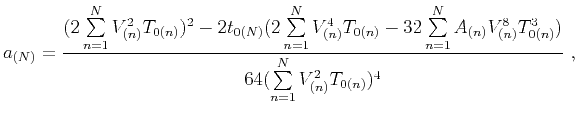
To test the accuracy of the previously suggested approximations for computing effective coefficients based on equation 62 against the exact expressions given in equations 45-47, we consider two three-layered models with parameters given in Table 2. The respective layer thicknesses are 0.25, 0.45, and 0.3  . We compute the quartic term (equation 36) at the offset radius of 1
and different azimuths.
. We compute the quartic term (equation 36) at the offset radius of 1
and different azimuths.
Table 2. Parameters of sample orthorhombic models under the notation of Tsvankin (1997) with the subscript denoting the normal direction to the corresponding plane: Model 1 (Weak anisotropy) parameters are extracted and modified from a layered model by (Ursin and Stovas, 2006; Stovas and Fomel, 2012) and Model 2 (Moderate-Strong anisotropy) parameters are modified from Schoenberg and Helbig (1997) and Tsvankin (1997).
Subsections
|
|
|
|
| Theory of interval traveltime parameter estimation in layered anisotropic media | |
|
Next: Comparison with the method
Up: Coefficients of traveltime expansion
Previous: Formulas for interval quartic
2017-04-14