|
|
|
|
Next: Discussion Up: Sun, Fomel, Zhu & Previous: -compensated LSRTM using the
|
|
|
|


|
|---|
|
vel,q
Figure 1. BP gas-cloud model. (a) A portion of the BP 2004 velocity model; (b) the corresponding quality factor |
|
|

|
|---|
|
shots
Figure 2. Prestack data with attenuation. A total of |
|
|


|
|---|
|
cref,imgd,imgc
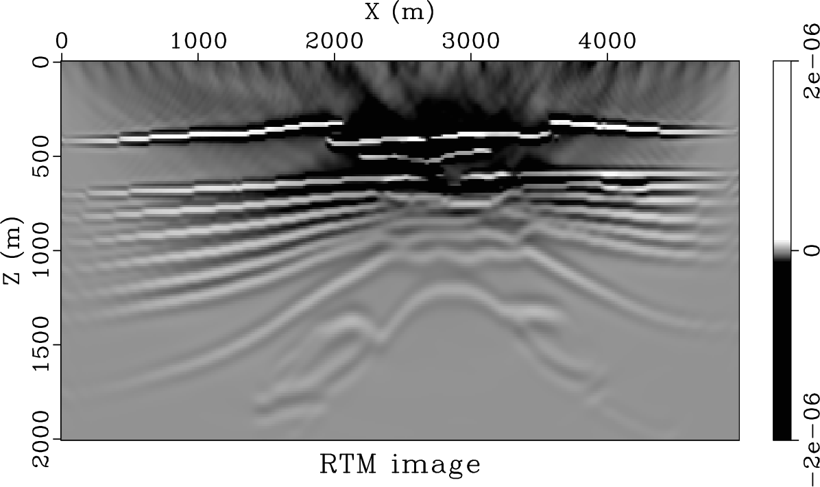
Figure 3. (a) The true reflectivity model; (b) image obtained by dispersion-only RTM without compensating for amplitude; (c) image obtained by |
|
|


|
|---|
|
img-n-5,img-n-15,img-n-30
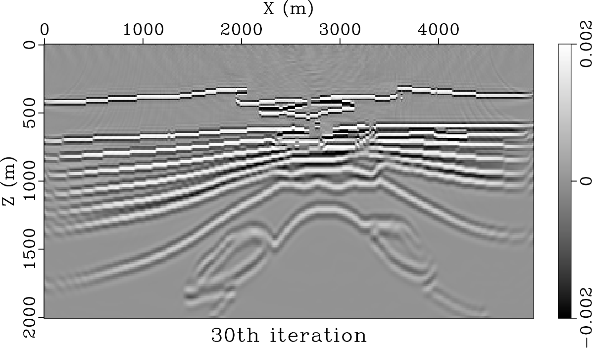
Figure 4. The results of the original LSRTM through iterations. (a) after |
|
|


|
|---|
|
img-v-5,img-v-15,img-v-30
Figure 5. The results of the LSRTM with Laplacian filter through iterations. (a) after |
|
|


|
|---|
|
img-c-5,img-c-15,img-c-30
Figure 6. The result of the proposed |
|
|


|
|---|
|
compare-n,compare-v,compare-c
Figure 7. Image traces extracted at |
|
|

|
|---|
|
conv
Figure 8. Convergence curves calculated by the |
|
|
To test the convergence rate of ![]() -LSRTM, we use a portion of the BP 2004 velocity model (Billette and Brandsberg-Dahl, 2004) and the corresponding
-LSRTM, we use a portion of the BP 2004 velocity model (Billette and Brandsberg-Dahl, 2004) and the corresponding ![]() model suggested by Zhu et al. (2014) (Figure 1). The model features a low-velocity, low-
model suggested by Zhu et al. (2014) (Figure 1). The model features a low-velocity, low-![]() area which is assumed to be caused by the presence of a gas chimney. The model has a spatial sampling rate of
area which is assumed to be caused by the presence of a gas chimney. The model has a spatial sampling rate of ![]() along both vertical and horizontal directions. A total of
along both vertical and horizontal directions. A total of ![]() shots with a spacing of
shots with a spacing of ![]() have been modeled with attenuation, and the source is a Ricker wavelet with
have been modeled with attenuation, and the source is a Ricker wavelet with ![]() peak frequency (Figure 2). Performing RTM without compensating for amplitude loss, i.e. using the dispersion-only operator, leads to an image corresponding to Figure 3b, which suffers from poor illumination below the gas chimney. In contrast,
peak frequency (Figure 2). Performing RTM without compensating for amplitude loss, i.e. using the dispersion-only operator, leads to an image corresponding to Figure 3b, which suffers from poor illumination below the gas chimney. In contrast, ![]() -RTM appears capable of recovering the amplitude at deeper reflectors (Figure 3c), but the image still exhibits some differences from the true reflectivity. Note that the dispersion-only RTM image and
-RTM appears capable of recovering the amplitude at deeper reflectors (Figure 3c), but the image still exhibits some differences from the true reflectivity. Note that the dispersion-only RTM image and ![]() -RTM image have the same phase but differ in amplitude. Next, we perform LSRTM (equation 19) and
-RTM image have the same phase but differ in amplitude. Next, we perform LSRTM (equation 19) and ![]() -LSRTM (equation 23) through a number of iterations. To test the separate effect of applying a Laplacian filter without compensating for attenuation, we also perform LSRTM with a Laplacian operator that removes low frequency artifacts. For fairness of comparison, all three methods are driven by the GMRES method, and because the tested model is small enough, they were not run in a restarted fashion. Using the original LSRTM (Figure 4), the inversion process attempts to remove low frequency noise and improve the illumination of deeper reflectors. However, at
-LSRTM (equation 23) through a number of iterations. To test the separate effect of applying a Laplacian filter without compensating for attenuation, we also perform LSRTM with a Laplacian operator that removes low frequency artifacts. For fairness of comparison, all three methods are driven by the GMRES method, and because the tested model is small enough, they were not run in a restarted fashion. Using the original LSRTM (Figure 4), the inversion process attempts to remove low frequency noise and improve the illumination of deeper reflectors. However, at ![]() th iteration, the reflector amplitude and sharpness beneath the attenuating area still have not been recovered. LSRTM with a Laplacian filter (Figure 5) achieves a somewhat sharper image, but because a Laplacian filter boosts high frequency components in the image, the reflectors beneath the attenuating zone remain poorly illuminated. In contrast, the proposed
th iteration, the reflector amplitude and sharpness beneath the attenuating area still have not been recovered. LSRTM with a Laplacian filter (Figure 5) achieves a somewhat sharper image, but because a Laplacian filter boosts high frequency components in the image, the reflectors beneath the attenuating zone remain poorly illuminated. In contrast, the proposed ![]() -LSRTM method (Figure 6) produces sharper reflectors with well-balanced illumination, especially in the area beneath the gas chimney using the same number of iterations. Note that the color scales used in all the three cases are kept the same as that of the true model (Figure 3a). Figure 7 compares the image traces extracted at
-LSRTM method (Figure 6) produces sharper reflectors with well-balanced illumination, especially in the area beneath the gas chimney using the same number of iterations. Note that the color scales used in all the three cases are kept the same as that of the true model (Figure 3a). Figure 7 compares the image traces extracted at ![]() from the
from the ![]() th iteration results against the true model. Clearly, the result obtained by the proposed
th iteration results against the true model. Clearly, the result obtained by the proposed ![]() -LSRTM best represents the true reflectivity, especially at deeper parts beneath the gas chimney (below
-LSRTM best represents the true reflectivity, especially at deeper parts beneath the gas chimney (below ![]() depth).
depth).
To measure the convergence rate, we calculate the model residual as the ![]() norm of the misfit between the model calculated at each iteration
norm of the misfit between the model calculated at each iteration ![]() and the true model
and the true model ![]() , normalized by the
, normalized by the ![]() norm of the true model:
norm of the true model:
|
|
|
|
