|
|
|
|
Fourier finite-difference wave propagation |
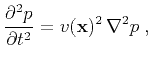
The acoustic wave equation is widely used in forward seismic modeling and reverse-time migration (Bednar, 2005; Etgen et al., 2009):
Equation 5 provides an elegant and efficient solution
in the case of a constant-velocity medium with the aid of FFT.
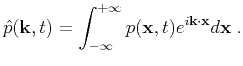
In the case of a variable-velocity medium,
equation 5 can provide an approximation by replacing ![]() with
with
![]() .
However, FFT can no longer be applied directly for
the inverse Fourier transform from the wavenumber domain back to the space domain.
To overcome this problem, Etgen and Brandsberg-Dahl (2009) propose a velocity interpolation method.
They present an implementation for isotropic, VTI (vertical transversely isotropic) and TTI (tilted transversely isotropic) media.
In the isotropic case, two FFTs can be sufficient.
For anisotropic media, more than one velocity parameter must be used.
Therefore, it is necessary to perform velocity interpolation
by combining different parameters and
computing the corresponding forward and inverse FFTs
for each of the velocity parameters, thus increasing the computational burden.
Other FFT-based solutions include the optimized separable approximation or OSA (Du et al., 2010; Song, 2001; Liu et al., 2009; Zhang and Zhang, 2009)
and the lowrank approximation (Fomel et al., 2010).
.
However, FFT can no longer be applied directly for
the inverse Fourier transform from the wavenumber domain back to the space domain.
To overcome this problem, Etgen and Brandsberg-Dahl (2009) propose a velocity interpolation method.
They present an implementation for isotropic, VTI (vertical transversely isotropic) and TTI (tilted transversely isotropic) media.
In the isotropic case, two FFTs can be sufficient.
For anisotropic media, more than one velocity parameter must be used.
Therefore, it is necessary to perform velocity interpolation
by combining different parameters and
computing the corresponding forward and inverse FFTs
for each of the velocity parameters, thus increasing the computational burden.
Other FFT-based solutions include the optimized separable approximation or OSA (Du et al., 2010; Song, 2001; Liu et al., 2009; Zhang and Zhang, 2009)
and the lowrank approximation (Fomel et al., 2010).
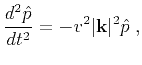
We propose an alternative approach.
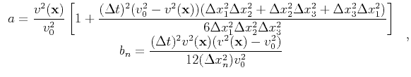
First, we adopt the following form of the right-hand side of equation 5 in the variable velocity case:
Equation 6 consists of two terms: the first term is independent of
![]() and only depends on
and only depends on
![]() .
For this part, we use inverse FFT to return to the space domain from the wavenumber domain.
For the remaining part, however, we can avoid phase shift in the wavenumber domain by implementing space shifts
through finite differences (approximation 7) with coefficients provided by equation 8.
This approach is analogous to the FFD method proposed by Ristow and Ruhl (1994) for one-way extrapolation in depth.
.
For this part, we use inverse FFT to return to the space domain from the wavenumber domain.
For the remaining part, however, we can avoid phase shift in the wavenumber domain by implementing space shifts
through finite differences (approximation 7) with coefficients provided by equation 8.
This approach is analogous to the FFD method proposed by Ristow and Ruhl (1994) for one-way extrapolation in depth.
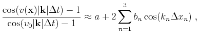
Figure 1 (a) shows approximations for
![]() by the 4th-order FD method (dash line) and pseudo-spectral method (dotted line). Figure 1 (b) shows approximations by the FFD method (2nd-order: dash line, 4th-order: dotted line).
The solid lines stand for the exact values for function
by the 4th-order FD method (dash line) and pseudo-spectral method (dotted line). Figure 1 (b) shows approximations by the FFD method (2nd-order: dash line, 4th-order: dotted line).
The solid lines stand for the exact values for function
![]() with true velocity:
with true velocity:
![]() (bottom solid line) and
(bottom solid line) and
![]() (top solid line), which indicates a significant velocity contrast (
(top solid line), which indicates a significant velocity contrast (![]() difference).
In this situation, all the approximations deviate from the exact solution as the wavenumber
difference).
In this situation, all the approximations deviate from the exact solution as the wavenumber ![]() becomes large.
However, the 4th-order FFD method approximates the exact solution with the most accuracy, as shown in the error plot (Figure 2).
In order to enhance the stability, one can suppress the wavefield at high wavenumbers for both pseudo-spectral and the FFD method.
becomes large.
However, the 4th-order FFD method approximates the exact solution with the most accuracy, as shown in the error plot (Figure 2).
In order to enhance the stability, one can suppress the wavefield at high wavenumbers for both pseudo-spectral and the FFD method.

|
|---|
|
cos-side1
Figure 1. Different approximations for |
|
|

|
|---|
|
diff1
Figure 2. Errors for different approximations for |
|
|
Assuming that
![]() and
and
![]() are already known, the time-marching algorithm can be specified as follows:
are already known, the time-marching algorithm can be specified as follows:
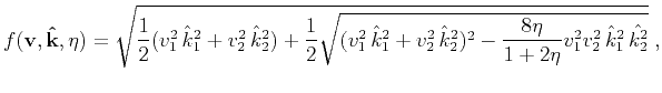
The FFD approach is not limited to the isotropic case.
In the case of transversally isotropic (TTI) media, the term
![]() on the left-hand side of equation 7,
can be replaced with the acoustic approximation (Fomel, 2004; Alkhalifah, 1998,2000),
on the left-hand side of equation 7,
can be replaced with the acoustic approximation (Fomel, 2004; Alkhalifah, 1998,2000),
where ![]() is the P-wave phase velocity in the symmetry plane,
is the P-wave phase velocity in the symmetry plane,
![]() is the P-wave phase velocity in the direction normal to the symmetry plane,
is the P-wave phase velocity in the direction normal to the symmetry plane,
![]() is the anisotropic elastic parameter (Alkhalifah and Tsvankin, 1995) related to Thomsen's elastic parameters
is the anisotropic elastic parameter (Alkhalifah and Tsvankin, 1995) related to Thomsen's elastic parameters ![]() and
and ![]() (Thomsen, 1986) by
(Thomsen, 1986) by
and
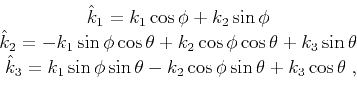
where ![]() is the tilt angle measured with respect to vertical and
is the tilt angle measured with respect to vertical and
![]() is the angle between the projection of the symmetry axis in the
horizontal plane and the original X-coordinate. The symmetry axis has
the direction of
is the angle between the projection of the symmetry axis in the
horizontal plane and the original X-coordinate. The symmetry axis has
the direction of
![]() .
.
Using these definitions, we develop a finite-difference approximation analogous to equation 7 for FFD in TTI media. The details of the derivation are given in the appendix. For the 2D TTI case, the corresponding FFD algorithm is as following:
![$ \displaystyle\frac{2[\cos(f(\mathbf{v_0},\mathbf{\hat{k}},\eta_0)\Delta t)-1]}{\vert\mathbf{\hat{k}}\vert^2}$](img66.png) to get
to get
|
|
|
|
Fourier finite-difference wave propagation |
![$\displaystyle 2\left[\cos(v_0\vert\mathbf{k}\vert\Delta t)-1\right]\left[\frac{...
...t\mathbf{k}\vert\Delta t)-1}{\cos(v_0\vert\mathbf{k}\vert\Delta t)-1}\right]\;,$](img25.png)