|
|
|
|
EMD-seislet transform |

|
|---|
|
demo,demo-fz
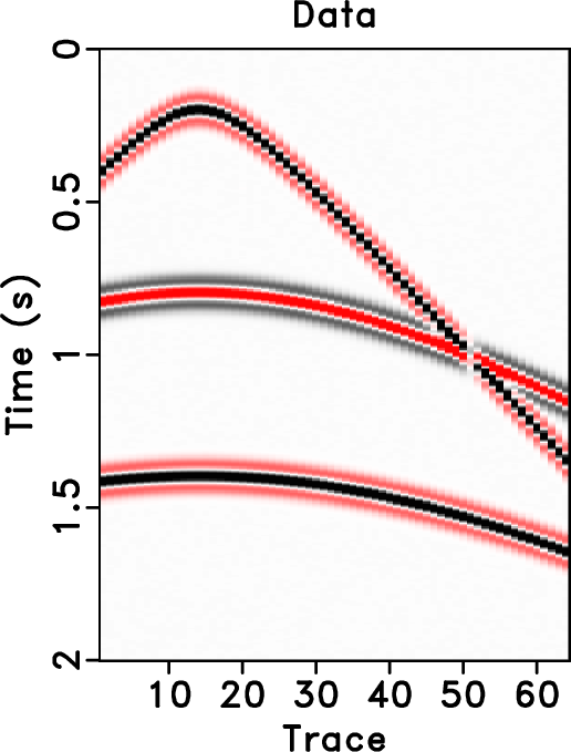
Figure 2. (a) Synthetic example with hyperbolic events. (b) |
|
|

|
|---|
|
demo-f1z-0,demo-f1z-seis-0,demo-dip1-0,demo-f2z-0,demo-f2z-seis-0,demo-dip2-0,demo-f3z-0,demo-f3z-seis-0,demo-dip3-0
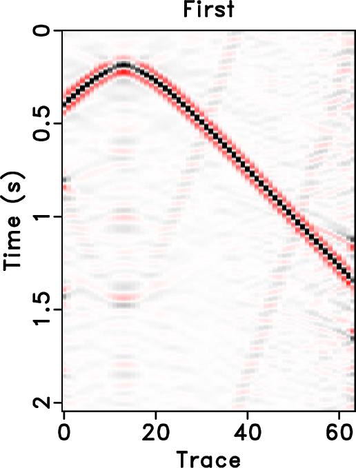
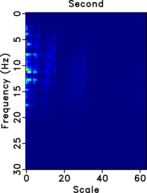
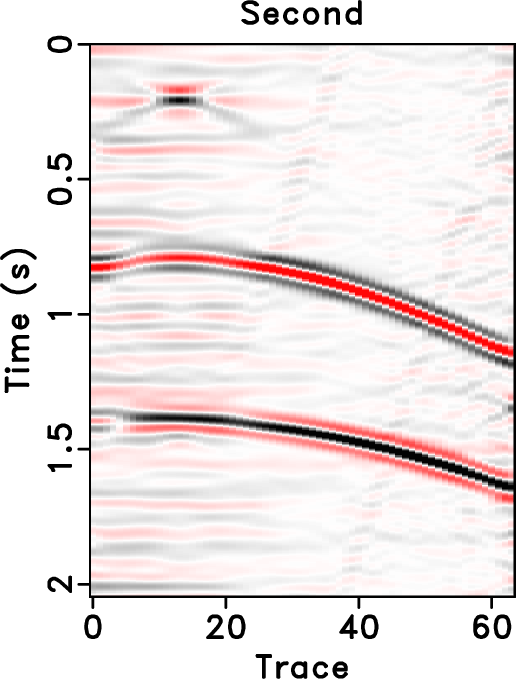
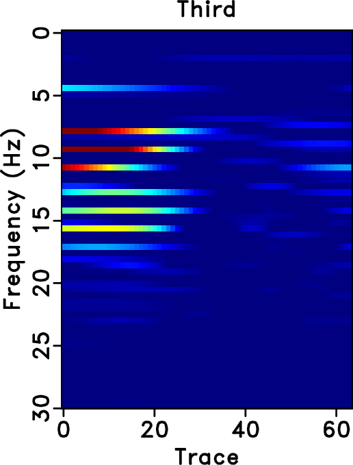
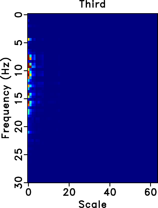
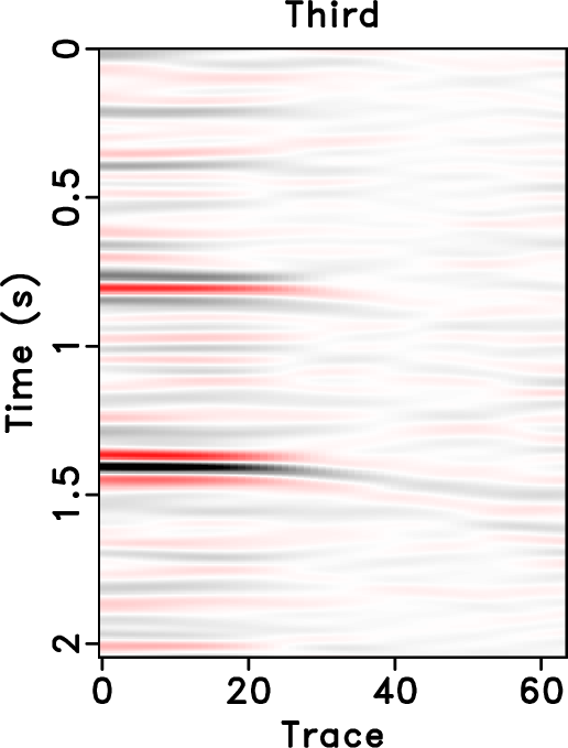
Figure 3. A demonstration of the EMD-seislet transform. The left column shows the decomposed |
|
|
The aforementioned 1D non-stationary seislet transform adapts to 1D signals that have smoothly variable frequency components since its compression performance is controlled by the predicting and updating procedures between the series elements according to a locally smooth modulation frequency. Correspondingly, when calculating the local frequency, we also assume the 1D signal to have smoothly variable frequency components.
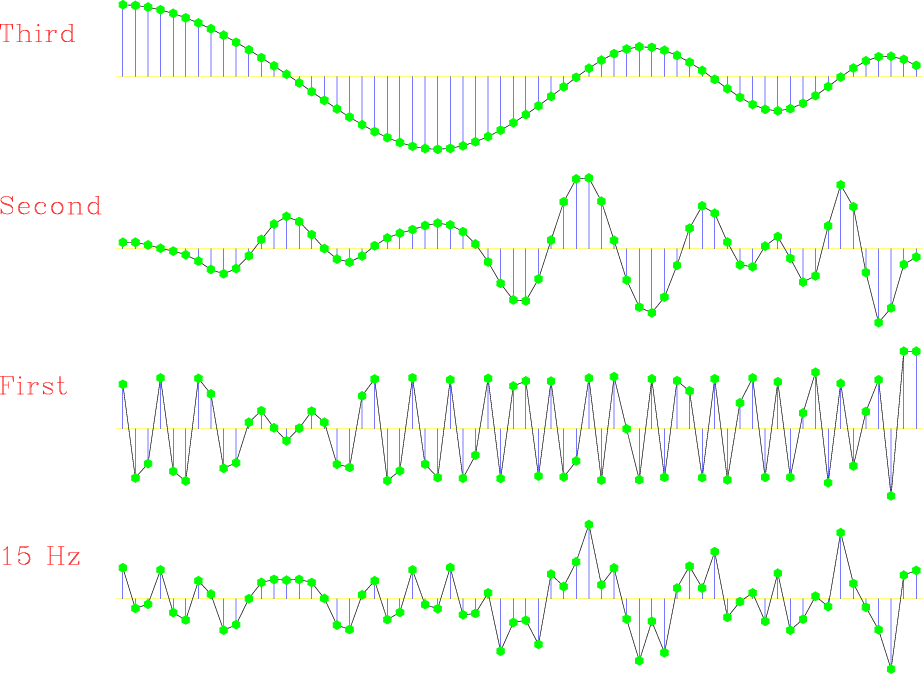
We call the combined FFT-EMD-seislet workflow the EMD-seislet transform. Figures 2 and 3 provide a detailed demonstration of the procedures involved in the EMD-seislet transform construction. Figure 2a shows a synthetic data with hyperbolic events. Figure 2b shows the ![]() spectrum of the synthetic data. Figure 4 shows a demonstration for preparing smoothly variable frequency components for each frequency slice using the EMD in the
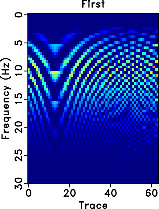
spectrum of the synthetic data. Figure 4 shows a demonstration for preparing smoothly variable frequency components for each frequency slice using the EMD in the ![]() domain. We can observe that each frequency slice in the
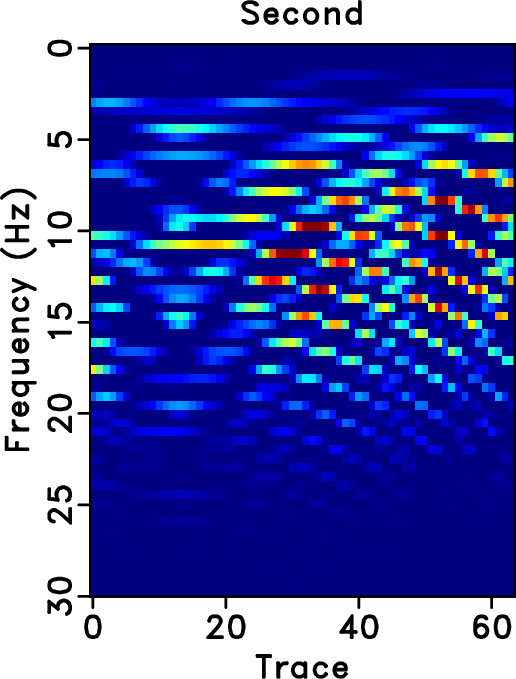
domain. We can observe that each frequency slice in the ![]() domain is highly non-stationary. After EMD decomposition, the three decomposed
domain is highly non-stationary. After EMD decomposition, the three decomposed ![]() domain components are shown in the left column of Figure 3. Each component now has smoothly non-stationary frequency slices. After 1D non-stationary seislet transforms, the three
domain components are shown in the left column of Figure 3. Each component now has smoothly non-stationary frequency slices. After 1D non-stationary seislet transforms, the three ![]() domain components become highly compressed. The middle column in Figure 3 shows the compressed
domain components become highly compressed. The middle column in Figure 3 shows the compressed ![]() domain using the 1D non-stationary seislet transform. The scale of the compressed coefficients is indicated by the horizontal axis. The right column in Figure 3 shows the reconstructed
domain using the 1D non-stationary seislet transform. The scale of the compressed coefficients is indicated by the horizontal axis. The right column in Figure 3 shows the reconstructed ![]() domain data from the decomposed and compressed components in the middle column. The three decomposed components correspond to different parts of the input signal.
domain data from the decomposed and compressed components in the middle column. The three decomposed components correspond to different parts of the input signal.
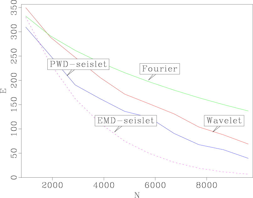
In order to compare the sparsity in compressing seismic data, we plot the reconstruction error curves with respect to the number of selected largest coefficients. The reconstruction error is defined as
![]() , where
, where
![]() denotes the largest
denotes the largest ![]() coefficients in the transform domain. The faster the curve decays, the sparser the corresponding transform domain will be. As shown in Figure 5, the EMD-seislet appears to be the sparsest compared with the PWD-seislet transform, wavelet transform, and Fourier transform.
coefficients in the transform domain. The faster the curve decays, the sparser the corresponding transform domain will be. As shown in Figure 5, the EMD-seislet appears to be the sparsest compared with the PWD-seislet transform, wavelet transform, and Fourier transform.
|
|---|
|
demo-fs-3
Figure 4. Demonstration of preparing the smoothly variable frequency components by EMD for the 15 Hz slice of the synthetic data in Figure 2a. |
|
|
|
|---|
|
sparse
Figure 5. Sparsity comparison. |
|
|
|
|
|
|
EMD-seislet transform |