|
|
|
|
First-break traveltime tomography with the double-square-root eikonal equation |
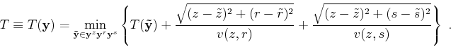
To simplify the analysis, we consider first the DSR branch as shown in Figure 1 and described by
equation 1. We assume a rectangular 2-D velocity model ![]() and thus a cubic 3-D prestack
volume
and thus a cubic 3-D prestack
volume ![]() with
with ![]() and
and ![]() axes having the same dimension as
axes having the same dimension as ![]() . After an Eulerian discretization of
both
. After an Eulerian discretization of
both ![]() and
and ![]() , we denote the grid spacing in
, we denote the grid spacing in ![]() as
as ![]() , and in
, and in ![]() ,
, ![]() and
and ![]() as
as ![]() .
.

|
|---|
|
update1
Figure 17. An implicit discretization scheme. The arrow indicates a DSR characteristic. Its root is located in the simplex |
|
|
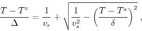
In Figure A-1, we study the traveltime at grid point
![]() and its relationship
with neighboring grid points
and its relationship
with neighboring grid points
![]() ,
,
![]() and
and
![]() with a semi-Lagrangian scheme. According to the geometry in
Figure 1, in the
with a semi-Lagrangian scheme. According to the geometry in
Figure 1, in the ![]() space the DSR characteristic (Duchkov and de Hoop, 2010) is straddled by
space the DSR characteristic (Duchkov and de Hoop, 2010) is straddled by
![]() .
.
In order to compute ![]() , we could continue along this characteristic up until its intersection with the simplex
, we could continue along this characteristic up until its intersection with the simplex
![]() . Suppose the intersection point is
. Suppose the intersection point is
![]() and
and ![]() 's are its barycentric coordinates, i.e.
's are its barycentric coordinates, i.e.
Defining the ratio in grid spacing as
![]() and denoting
and denoting ![]() and
and
![]() , equation A-2 can be re-written with the barycentric coordinates in
A-1 as
, equation A-2 can be re-written with the barycentric coordinates in
A-1 as
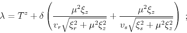
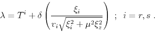
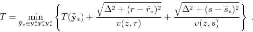
To explore the causal properties of equation A-3, we first assume that the minimum is attained at
some
![]() such that
such that ![]() for
for ![]() . From the Kuhn-Tucker optimality conditions (Kuhn and Tucker, 1951), there exists a Lagrange
multiplier
. From the Kuhn-Tucker optimality conditions (Kuhn and Tucker, 1951), there exists a Lagrange
multiplier ![]() such that
such that
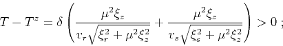
A direct substitution from equations A-6 and A-7 results in
If there is no real root or none of the real roots satisfy A-8, the minimizer
![]() can not lie in the interior of simplex
can not lie in the interior of simplex
![]() and at least one of the
and at least one of the ![]() s
must be zero. If
s
must be zero. If ![]() , it is easy to show that one of the other barycentric coordinates is also zero and
equation A-3 simplifies to
, it is easy to show that one of the other barycentric coordinates is also zero and
equation A-3 simplifies to
We note that the one-sided update A-14 could be considered a special case of two-sided updates: if
![]() (or
(or ![]() ), then A-14 becomes equivalent to A-12 (or, respectively,
A-13). Similarly, the two-sided updates can be viewed as special versions of the three-sided one:
e.g., if
), then A-14 becomes equivalent to A-12 (or, respectively,
A-13). Similarly, the two-sided updates can be viewed as special versions of the three-sided one:
e.g., if
![]() , then A-9 becomes equivalent to A-13. This means
that the causal criteria for formulas A-9, A-12 and A-13 can be relaxed (the
inequalities do not have to be strict). This relaxation is used to streamline the update strategy in the
Numerical Implementation section.
, then A-9 becomes equivalent to A-13. This means
that the causal criteria for formulas A-9, A-12 and A-13 can be relaxed (the
inequalities do not have to be strict). This relaxation is used to streamline the update strategy in the
Numerical Implementation section.
In Figure A-1 and the corresponding semi-Lagrangian discretization A-2, the ray-path
is linearly approximated up to its intersection with the simplex
![]() at a
priori unknown depth
at a
priori unknown depth
![]() . An alternative explicit semi-Lagrangian discretization can be
obtained in the spirit of Figure 1 by tracing the ray up to the pre-specified depth
. An alternative explicit semi-Lagrangian discretization can be
obtained in the spirit of Figure 1 by tracing the ray up to the pre-specified depth ![]() .
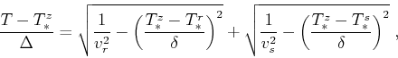
In Figure A-2, we consider the DSR characteristic being straddled by
.
In Figure A-2, we consider the DSR characteristic being straddled by
![]() , where
, where
![]() ,
,
![]() and
and
![]() . Denoting
. Denoting
![]() for the intersection point between DSR characteristic
and simplex
for the intersection point between DSR characteristic
and simplex
![]() , we obtain the following discretization:
, we obtain the following discretization:

|
|---|
|
update2
Figure 18. An explicit discretization scheme. Compare with Figure A-1. The arrow again depicts a DSR characteristic with its root confined in the simplex |
|
|
Compared with equation A-9, equation A-16 does not
require solving a polynomial equation. Moreover, ![]() depends only on
values in lower z-slices, which means that the system of equations can be solved in a single sweep in the
depends only on
values in lower z-slices, which means that the system of equations can be solved in a single sweep in the ![]() direction. Unfortunately, despite this efficiency on a fixed grid, the explicit discretization has a major
disadvantage stemming from the requirement that the characteristic should be straddled by
direction. Unfortunately, despite this efficiency on a fixed grid, the explicit discretization has a major
disadvantage stemming from the requirement that the characteristic should be straddled by
![]() .
This imposes an upper bound on
.
This imposes an upper bound on ![]() based on the slope of the diving wave. Moreover, since every diving ray is
horizontal at its lowest point, the convergence is possible only if
based on the slope of the diving wave. Moreover, since every diving ray is
horizontal at its lowest point, the convergence is possible only if ![]() under mesh refinement. In
practice, this means that the results are meaningful only if
under mesh refinement. In
practice, this means that the results are meaningful only if ![]() is significantly smaller than
is significantly smaller than ![]() . We
note that restrictive stability conditions also arise for time-dependent Hamilton-Jacobi equations of optimal
control, where sufficiently strong inhomogenieties can make nonlinear/implicit schemes preferable to the usual
linear/explicit approach (Vladimirsky and Zheng, 2013).
. We
note that restrictive stability conditions also arise for time-dependent Hamilton-Jacobi equations of optimal
control, where sufficiently strong inhomogenieties can make nonlinear/implicit schemes preferable to the usual
linear/explicit approach (Vladimirsky and Zheng, 2013).
The above analysis also applies to the first branch of the DSR eikonal equation in Figure 2.
However, in the discretized ![]() domain, the slowness vectors at
domain, the slowness vectors at ![]() and
and ![]() are always
aligned in the
are always
aligned in the ![]() direction, either upward or downward. For this reason, there is no DSR characteristic that
accounts for the second and third scenarios. We will refer to the first and last branches in
Figure 2 as causal branches of DSR eikonal equation, and the left-over two as
non-causal branches.
direction, either upward or downward. For this reason, there is no DSR characteristic that
accounts for the second and third scenarios. We will refer to the first and last branches in
Figure 2 as causal branches of DSR eikonal equation, and the left-over two as
non-causal branches.

|
|---|
|
search
Figure 19. When slowness vectors at |
|
|
Note that when the slowness vectors at ![]() and
and ![]() are pointing in opposite directions, there must be at least
one intersection of the ray-path with the
are pointing in opposite directions, there must be at least
one intersection of the ray-path with the ![]() depth level in-between. As shown in Figure A-3, ray
segments between these intersections fall into the category of causal branches. Thus a search process for the
intersections is sufficient in recovering the non-causal branches during forward modeling. Moreover, because we
are interested in first-breaks only, the minimum traveltime requirement allows us to search for only one
intersection, such as
depth level in-between. As shown in Figure A-3, ray
segments between these intersections fall into the category of causal branches. Thus a search process for the
intersections is sufficient in recovering the non-causal branches during forward modeling. Moreover, because we
are interested in first-breaks only, the minimum traveltime requirement allows us to search for only one
intersection, such as ![]() denoted in Figure A-3:
denoted in Figure A-3:
Unfortunately, this search routine induces considerable computational cost. Moreover, we note that, under a dominant diving waves assumption, the first DSR branch, despite being causal, becomes useless if A-17 is turned-off.
|
|
|
|
First-break traveltime tomography with the double-square-root eikonal equation |