|
|
|
|
An open-source Matlab code package for improved rank-reduction 3D seismic data denoising and reconstruction |
Next: Conclusions Up: An open-source Matlab code Previous: Code description
|
|
|
|
An open-source Matlab code package for improved rank-reduction 3D seismic data denoising and reconstruction |
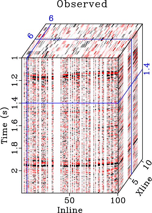
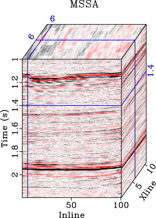
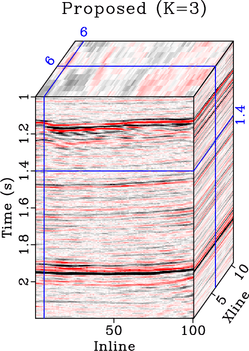
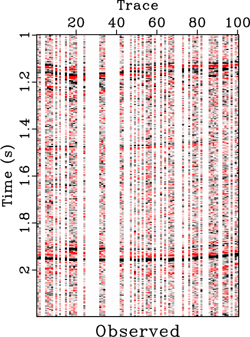
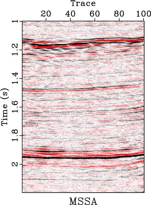
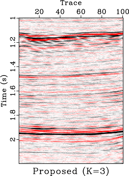
The field data example is shown in Figure 5. In this example, we do not know the true answer and thus we can not judge the reconstruction and denoising performance by comparing the final results with the true model as used in the synthetic example. Instead, we can only judge the performance by the spatial coherency of the reconstructed data. Figure 5a shows the observed noisy and incomplete data, which has been binned to regular grids. There are about 50% missing traces in this example. Figures 5b and 5c show the final results using the traditional and proposed improved MSSA algorithms. Figures 5d, 5e, and 5f show the 4th crossline slices of Figures 5a, 5b, and 5c, respectively. It can be seen that both methods can effectively reconstruct the missing data and attenuate the strong random noise, but the proposed improved MSSA algorithm can obtain even better performance since the events are more spatially coherent. It is worth mentioning that since there is no true answer for the field data example, it is hard to use quantitive measure to compare the performance of different approaches. The visual observation on the spatial coherency, instead, is the most effective and straightforward way.
Both examples are processed using the introduced Matlab packages. The binary files output from the Matlab packages are then put into the Madagascar platform to generate the final figures shown in Figures 1-5.
|
|---|
|
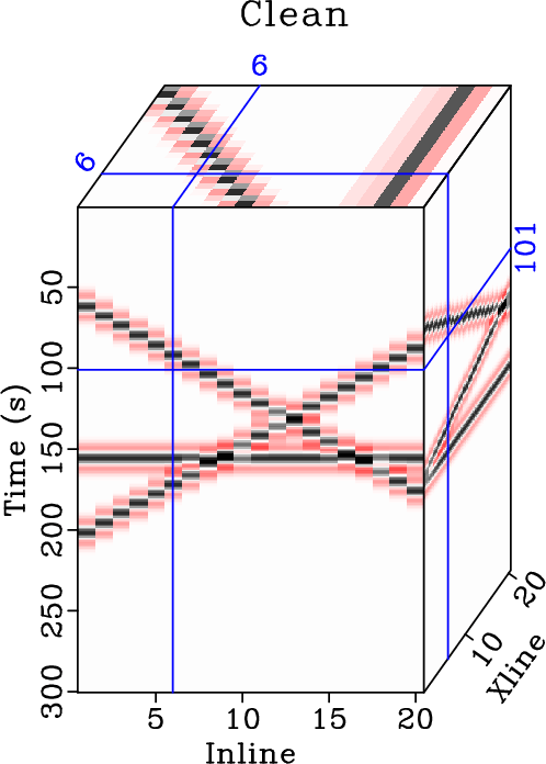
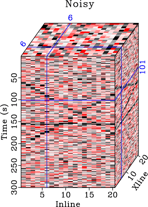
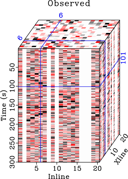
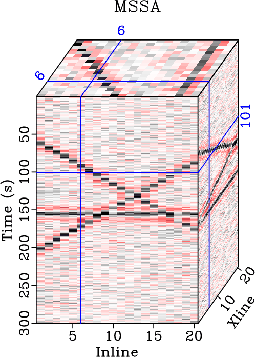
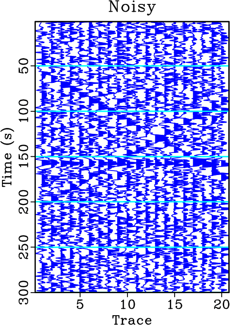
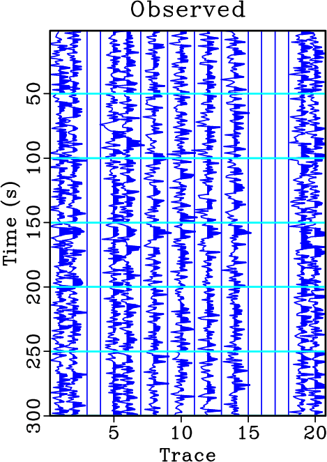
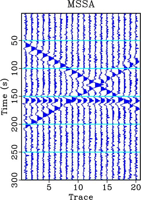
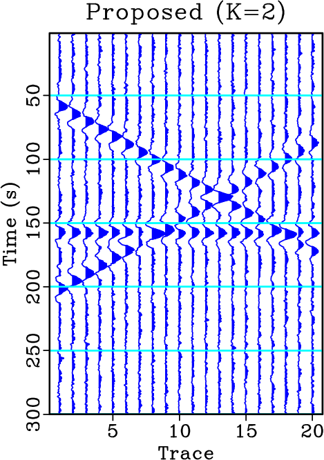
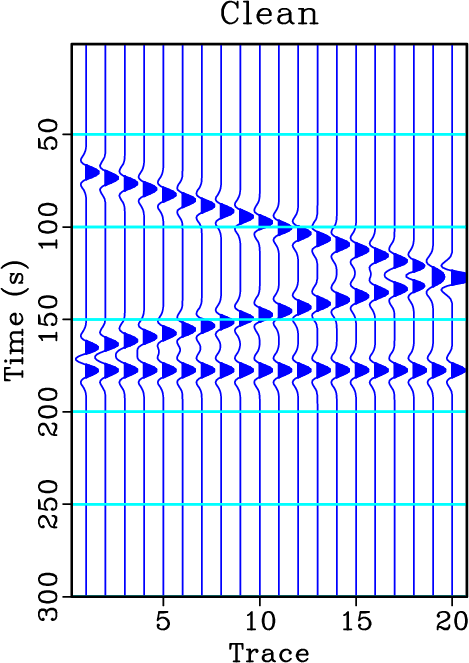
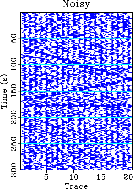
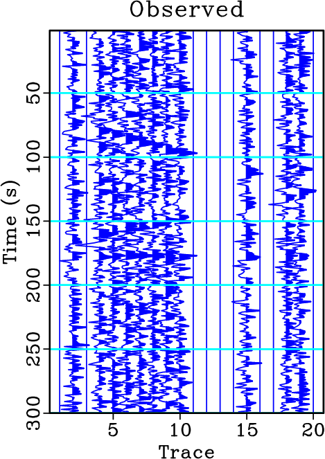
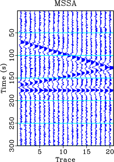
synth-clean,synth-noisy,synth-obs,synth-mssa,synth-dmssa2
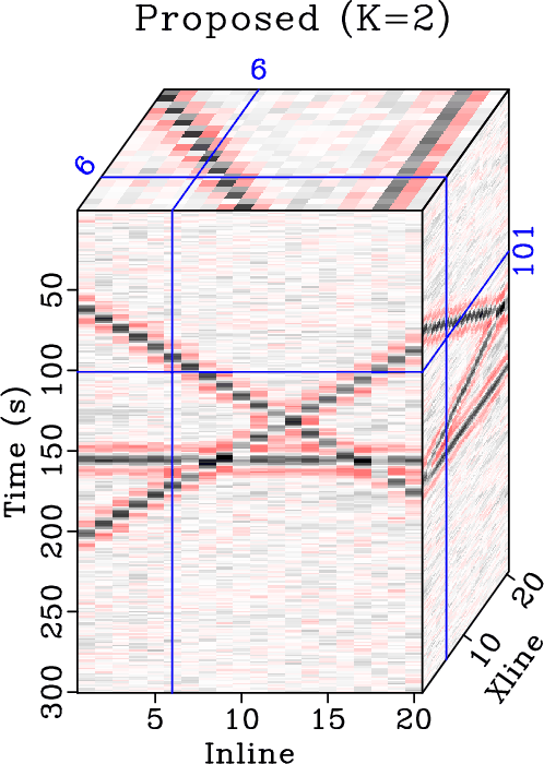
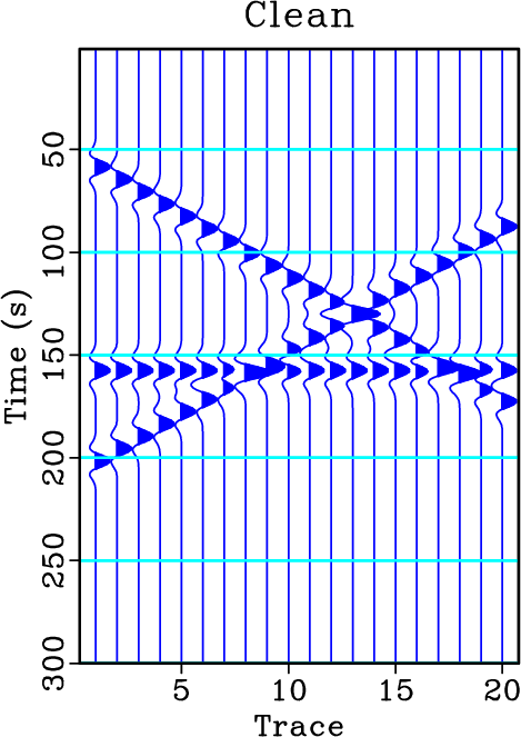
Figure 1. (a) Clean data. (b) Noisy data. (c) Observed data with 50% missing traces. (d) Denoised and reconstructed using the MSSA method. (e) Denoised and reconstructed using the proposed approach ( |
|
|
|
|---|
|
synth-dmssa1,synth-dmssa
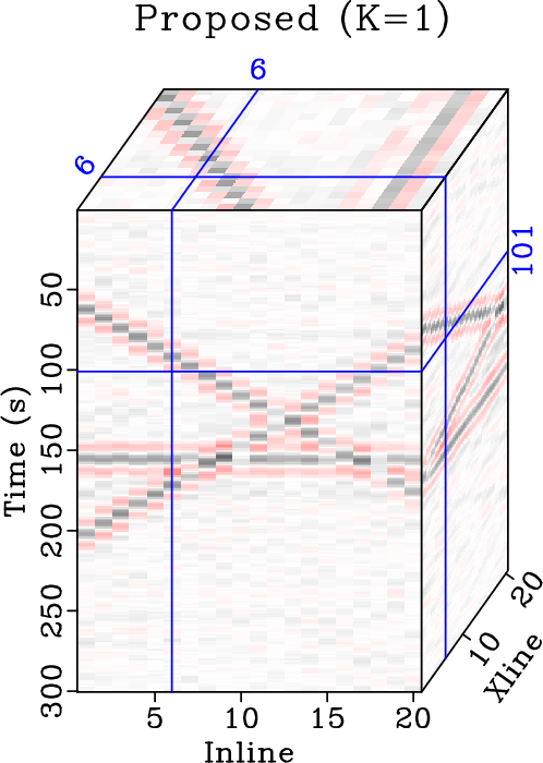
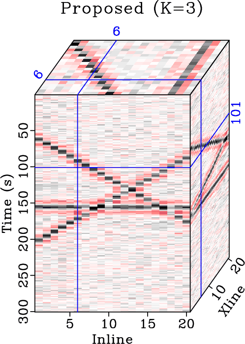
Figure 2. (a) Denoised and reconstructed data using the proposed approach when |
|
|
|
|---|
|
synth-s-clean,synth-s-noisy,synth-s-obs,synth-s-mssa,synth-s-dmssa2
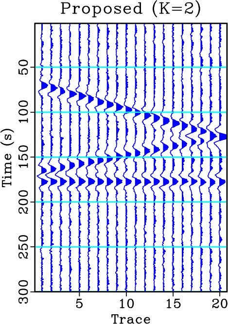
Figure 3. Single slice comparison (5th crossline section). (a) Clean data. (b) Noisy data. (c) Observed data with 50% missing traces. (d) Denoised and reconstructed using the MSSA method. (e) Denoised and reconstructed data using the proposed approach ( |
|
|
|
|---|
|
synth-s-clean-i,synth-s-noisy-i,synth-s-obs-i,synth-s-mssa-i,synth-s-dmssa2-i
Figure 4. Single slice comparison (5th inline section). (a) Clean data. (b) Noisy data. (c) Observed data with 50% missing traces. (d) Denoised and reconstructed using the MSSA method. (e) Denoised and reconstructed using the proposed approach ( |
|
|
|
|---|
|
field-obs,field-mssa,field-dmssa,field-s-obs,field-s-mssa,field-s-dmssa
Figure 5. (a) Observed field data (binned to the regular grid). (b) Reconstructed data using the MSSA method. (c) Reconstructed data using the DMSSA method. (d) 4th crossline slice of the observed data. (e) 4th crossline slice of the MSSA reconstructed data. (f) 4th crossline slice of the reconstructed data using the proposed approach. |
|
|
|
|
|
|
An open-source Matlab code package for improved rank-reduction 3D seismic data denoising and reconstruction |