|
|
|
|
Dip-separated structural filtering using seislet transform and adaptive empirical mode decomposition based dip filter |
Next: Dip separation using adaptive Up: Method Previous: Method
|
|
|
|
Dip-separated structural filtering using seislet transform and adaptive empirical mode decomposition based dip filter |
The above prediction and update operators can be defined as follows:
It is easier for understanding the seislet transform by extending the regular wavelet transform to seislet transform. For example, in the simplest case of Haar transform, the Z-transform domain prediction filter for the Haar wavelet transform is
Although the seislet transform has been demonstrated to have a better compression performance for seismic data (Fomel and Liu, 2010) than other alternatives given that an fairly acceptable local slope field can be obtained, the limitation is that it heavily depends on the estimation of local slope. As shown in equations 5 and 6, the only difference between the seislet transform and the traditional second-generation wavelet is the prediction operator. When the plane-wave destruction operator can obtain an accurate local slope, e.g. where seismic reflections are spatially coherent and no dip conflicts exist, the seismic data can be compressed by the seislet transform with a high compression ratio. However, when the local slope is not appropriately estimated, e.g. the seismic profile is very complicated, the seislet transform will not obtain a better compression result than traditional wavelet transform.
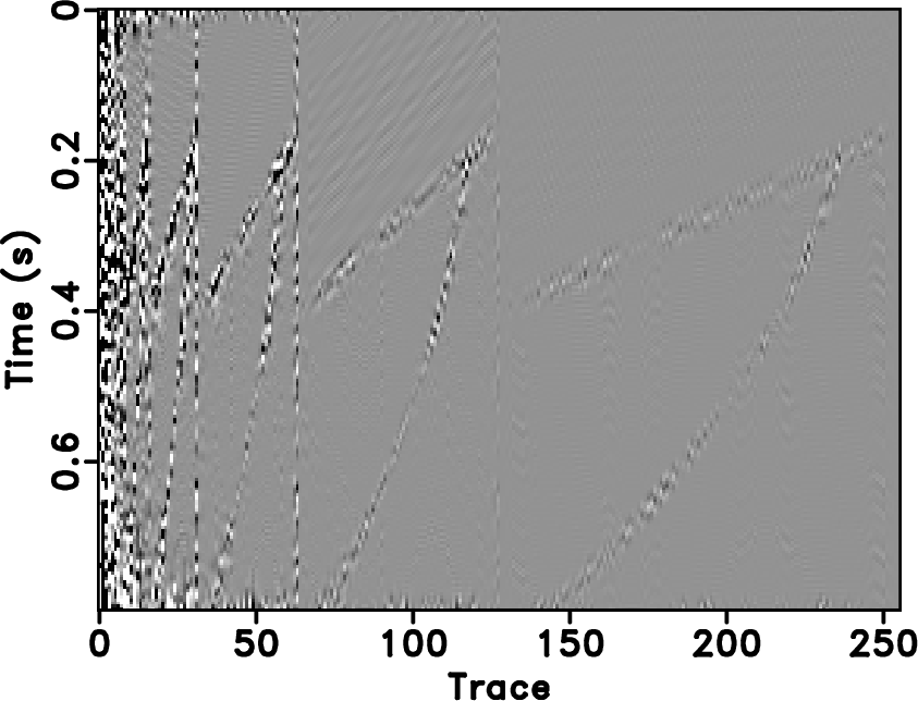
Figures 1, 2 and 3 demonstrate the dip-dependence problem of the seislet transform. Figure 1a shows the well-known Sigmoid model (Claerbout, 2010). Figure 1b shows the dip estimation result using plane-wave destruction with the best parameters selection. The dip estimation is very accurate in that it is consistent with the structure and causes a sparse compression in the seislet domain, as shown in Figure 1c. I treat this dip estimation as the true local slope as a reference for the comparison shown later. And the corresponding seislet domain is treated as the true seislet domain. In order to test the compression performance using different slope estimations, I smooth the true local slope with different smoothing radii. The longer smoothing radius is, the higher error exists in the local slope. Figure 2 shows three local slope maps with different smoothing radii and their corresponding seislet domains. When the smoothing radius is 50, the slope map is still very similar to the true local slope, and the seislet transform can still get an acceptable result, though much worse than the true seislet domain. When the smoothing radius increases to 100, the slope map cannot indicate the general structure of seismic data, the seislet transform gets an even worse result, as shown in Figure 2d. When the smoothing radius is 250, the slope map is nearly zero, and the seislet domain is not sparse any more. In order to numerically compare the sparseness, I sort the seislet domain coefficients according to the normalized amplitude and draw their magnitude-decreasing diagrams, as shown in Figure 3. In Figure 3, the faster the coefficients decrease, the sparser the seislet domain is. From this figure, I observe that the coefficients in the true seislet domain decreases fastest, and as the smoothing radius becomes longer and longer, the coefficients decrease slower and slower. I also plot the magnitude-decreasing diagram of the curvelet transform, which lays between ![]() and
and ![]() when
when ![]() is small and becomes almost constant when
is small and becomes almost constant when ![]() is large. It can be inferred that even when the local slope contains significant error, the seislet domain is still sparser than the curvelet domain. In field data processing, when the subsurface structure is complicated, however, plane-wave destruction operator cannot obtain acceptable local slope estimation because of the dip conflicts, which makes the seislet domain not optimally sparse. Thus, for these seismic profiles, the performance of conventional seislet thresholding will be deteriorated.
is large. It can be inferred that even when the local slope contains significant error, the seislet domain is still sparser than the curvelet domain. In field data processing, when the subsurface structure is complicated, however, plane-wave destruction operator cannot obtain acceptable local slope estimation because of the dip conflicts, which makes the seislet domain not optimally sparse. Thus, for these seismic profiles, the performance of conventional seislet thresholding will be deteriorated.


|
|---|
|
sig,dip0,slet0
Figure 1. (a) Synthetic data. (b) True local slope. (c) True seislet domain. |
|
|


|
|---|
|
dip1,slet1,dip2,slet2,dip3,slet3
Figure 2. Smoothed local slope maps using different smoothing radii (SR) and the corresponding seislet domain. (a) Local slope map with |
|
|

|
|---|
|
sigcoef
Figure 3. Seislet domain coefficients decreasing diagrams, compared with the curvelet domain coefficients decreasing diagram. |
|
|
|
|
|
|
Dip-separated structural filtering using seislet transform and adaptive empirical mode decomposition based dip filter |
![$\displaystyle \mathbf{P}\left[\mathbf{e}\right]_k=\left(\mathbf{P}^{(+)}_k\left[\mathbf{e}_{k-1}\right]+\mathbf{P}^{(-)}_k\left[\mathbf{e}_k\right]\right)/2,$](img18.png)
![$\displaystyle \mathbf{U}\left[\mathbf{r}\right]_k=\left(\mathbf{P}^{(+)}_k\left[\mathbf{r}_{k-1}\right]+\mathbf{P}^{(-)}_k\left[\mathbf{r}_k\right]\right)/4,$](img19.png)