Post-stack velocity analysis by separation and imaging of seismic diffractions

Channel detection

zovel,zovol
Figure 8. 3-D synthetic test. (a) Synthetic velocity model for a channelized reservoir. (b) Modeled zero-offset data.

xdip,xpwd
Figure 9. Diffraction separation for the 3-D synthetic test from Figure 8. (a) Dominant in-line slope estimated by plane-wave destruction. (b) Diffractions separated from the data.

zomig,pwmig
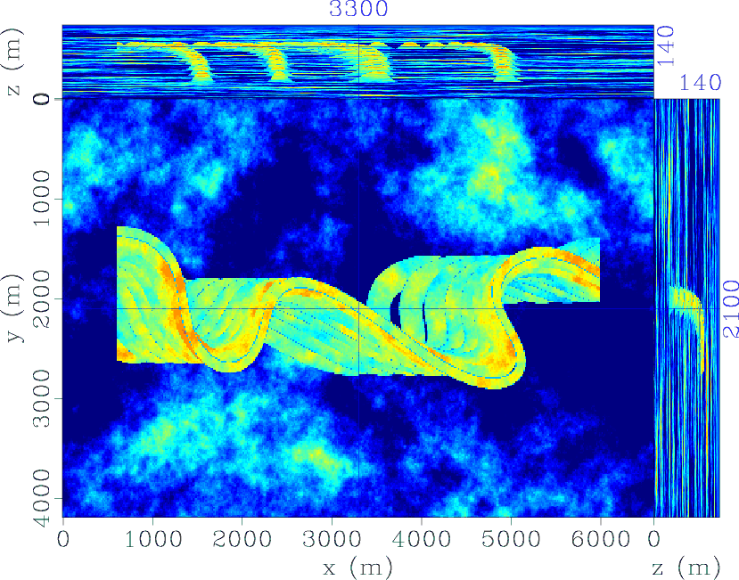
Figure 10. Depth migration of the 3-D synthetic test data. (a) Migrated data. (b) Migrated diffractions.

The third example is a 3-D synthetic dataset. The velocity model was designed to simulate a complex sand channel geometry in a deep-water clastic reservoir (Figure 8a). Including an overburden with stochastically generated velocity fluctuations on top of the reservoir model, we generated zero-offset data shown in Figure 8b. The data contain reflections from continuous parts of the model and numerous diffractions generated by the channel edges. Separating diffractions using in-line plane-wave destruction (Figure 9), we compare depth-migrated images of the original data and of the separated diffractions (Figure 10). The fine details of the stacked channel geometry are revealed by diffraction imaging.

Post-stack velocity analysis by separation and imaging of seismic diffractions