Post-stack velocity analysis by separation and imaging of seismic diffractions

Imaging diffractions

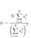
How can one detect the spatially-variable velocity necessary for focusing of different diffraction events? A good measure of focusing is the varimax norm used by Wiggins (1978) for minimum-entropy deconvolution and by Levy and Oldenburg (1987) for zero-phase correction. The varimax norm is defined as

$$\phi = \frac{\displaystyle N\,\sum_{i=1}^N s_i^4}{\displaystyle \left(\sum_{i=1}^{N} s_i^2\right)^2}\;,$$ (1)

where $s_i$ are seismic signal amplitudes inside a window of size $N$. Varimax is simply related to kurtosis of zero-mean signals.

Rather than working with data windows, we turn focusing into a continuously variable attribute using the technique of local attributes (Fomel, 2007a). Noting that the correlation coefficient of two sequences $a_i$ and $b_i$ is defined as

$$c[a,b] = {\frac{\displaystyle \sum_{i=1}^N a_i\,b_i}{\displaystyle \sqrt{\sum_{i=1}^N a_i^2\,\sum_{i=1}^N b_i^2}}}$$ (2)

and the correlation of $a_i$ with a constant is

$$c[a,1] = {\frac{\displaystyle \sum_{i=1}^N a_i}{\displaystyle \sqrt{N\,\sum_{i=1}^N a_i^2}}}\;,$$ (3)

one can interpret the varimax measure in equation 1 as the inverse of the squared correlation coefficient between $s_i^2$ and a constant: $\phi = 1/c[s^2,1]^2$. Well-focused signals have low correlation with a constant and correspondingly high varimax.

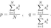
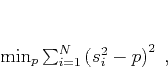
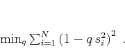
Going further toward a continuously variable focusing attribute, notice that the squared correlation coefficient can be represented as the product of two quantities $c[s^2,1]^2 = p\,q$, where

$$p=\frac{\displaystyle \sum_{i=1}^N s_i^2}{\displaystyle N}\;... ...style \sum_{i=1}^N s_i^2}{\displaystyle \sum_{i=1}^N s_i^4}\;.$$ (4)

Furthermore, $p$ is the solution of the least-squares minimization problem

$$\min_p \sum_{i=1}^N \left(s_i^2 - p\right)^2\;,$$ (5)

and $q$ is the solution of the least-squares minimization

$$\min_q \sum_{i=1}^N \left(1 - q\,s_i^2\right)^2\;.$$ (6)

This allows us to define a continuously variable attribute $\phi_i$ by using continuously variable quantities $p_i$ and $q_i$, which are defined as solutions of regularized optimization problems

$$\min_{p_i} \left(\sum_{i=1}^N \left(s_i^2 - p_i\right)^2 + R\left[p_i\right]\right)\;,$$ (7)

$$\min_{q_i} \left(\sum_{i=1}^N \left(1 - q_i\,s_i^2\right)^2 + R\left[q_i\right]\right)\;,$$ (8)

where $R$ is a regularization operator designed to avoid trivial solutions by enforcing a desired behavior (such as smoothness). Shaping regularization (Fomel, 2007b) provides a particularly convenient method for enforcing smoothing in an iterative optimization scheme.

We apply the local focusing measure to obtain migration-velocity panels for every point in the image. First, we follow the procedure outlined in the previous section to replace a stacked or zero-offset section with a section containing only separated diffractions. Next, we migrate the data multiple times with different migration velocities. This is accomplished by velocity continuation (Fomel, 2003a), a method that performs time-migration velocity analysis by continuing seismic images in velocity with the process also called ``image waves'' (Hubral et al., 1996). The velocity continuation theory (Fomel, 2003b) shows that one can accomplish time migration with a set of different velocities by making differential steps in velocity similarly to the method of cascaded migrations (Larner and Beasley, 1987) but described and implemented as a continuous process. While comparable in theory to an ensemble of Stolt migrations (Fowler, 1984; Mikulich and Hale, 1992), velocity continuation has the advantage of working directly in the image domain. It is implemented with an efficient and robust algorithm based on the Fast Fourier Transform.

Finally, we compute $\phi_i$ for every sample point in each of the migrated images. Thus, $N$ in equations 7 and 8 refers to the total number of sample points in an image. The output is focusing image gathers (FIGs), exemplified in Figure 1. A FIG is analogous to a conventional migration-velocity analysis panel and suitable for picking migration velocities. The main difference is that the velocity information is obtained from analysis of diffraction focusing as opposed to semblance of flattened image gathers used in prestack analysis.

Post-stack velocity analysis by separation and imaging of seismic diffractions