|
|
|
|
Elastic wave-vector decomposition in heterogeneous anisotropic media |
 |
|||
 |
|||
 ,
,
 |
(23) |
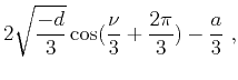
 |
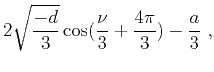
(24) |

|
|---|
|
ortoctant,orthos
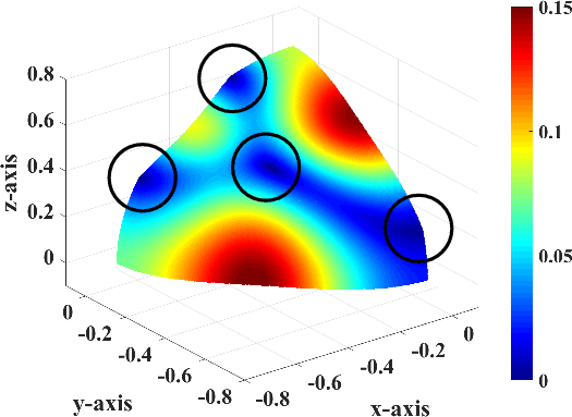
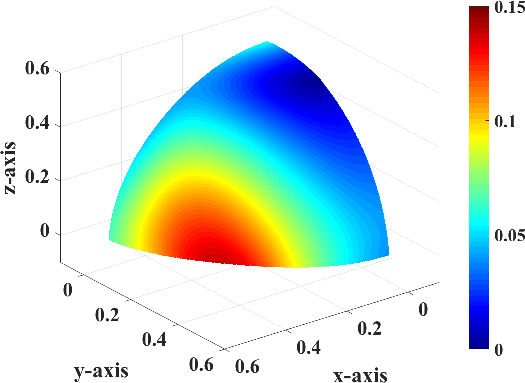
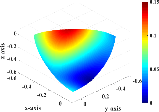
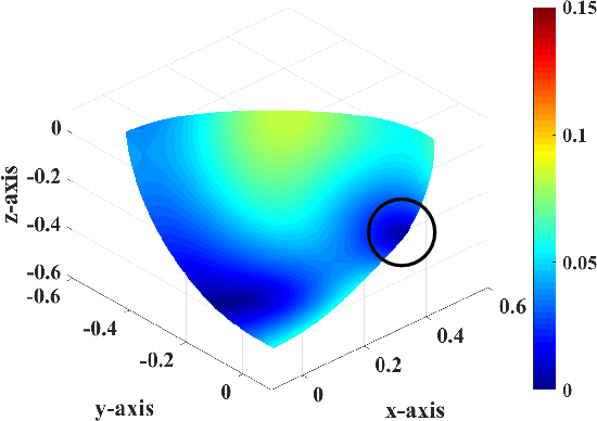
Figure 3. a) Polarization vectors in the orthorhombic model of S1 (blue) and S2 (red) plotted on phase slowness surfaces to show how they rapidly rotate in the vicinity of point singularities. b) |
|
|
|
|---|
|
t090p090s,t090p90180s,t090p180270s,t090p270360s
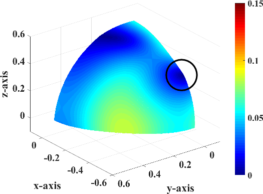
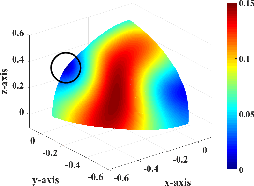
Figure 4. |
|
|

|
|---|
|
t90180p090s,t90180p90180s,t90180p180270s,t90180p270360s
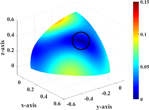
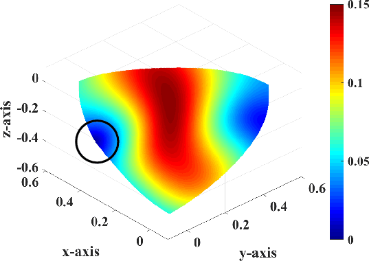
Figure 5. |
|
|
|
|
|
|
Elastic wave-vector decomposition in heterogeneous anisotropic media |