|
|
|
|
Iterative deblending of simultaneous-source seismic data using seislet-domain shaping regularization |
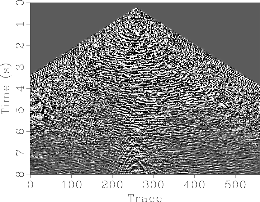
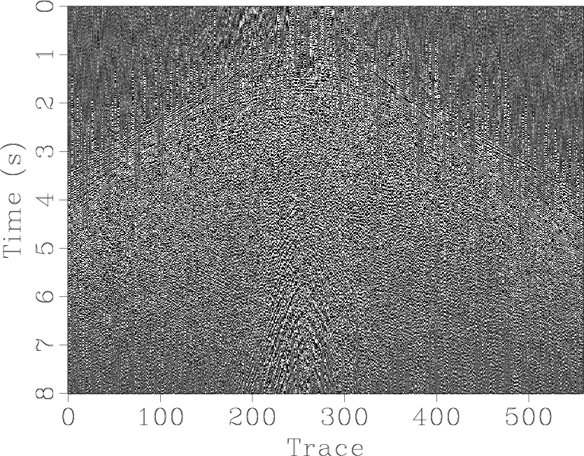
Finally, we use a field data example to further test the effectiveness for our proposed algorithm. The field data is similar in appearance to the previous synthetic example. Because of the previous test, we only used seislet-domain soft thresholding as the shaping operator.
The two blended data are shown in Figures 12a and 12b and appear noisy.
After 30 iterations of seislet-domain soft thresholding, the deblending results are shown in Figures 12d and 12c. The intense interference in the shallow part has been removed to a large extent. The deep-water reflection becomes much clearer because of a significant drop in the noise energy for the whole profile. From the noise sections, we can observe only a small amount of ground roll, which is analogous to the results of the previous synthetic test, and a even less amount of direct waves and shallow part horizontal reflections, which is not significant. The ![]() defined in equation 8 obtained an increase from 1.00
defined in equation 8 obtained an increase from 1.00 ![]() to 5.50
to 5.50 ![]() for the first source and from 0.83
for the first source and from 0.83 ![]() to 5.50
to 5.50 ![]() for the second source. The error sections for this field data test are not given since the unblended data for this test contain much random noise, which can not be estimated.
However, from the point of view of random noise attenuation, which is concerned with the signal content of the denoised section and the randomness of the noise section, the deblending result of the field data test is acceptable. In this case, the percentage we use for seislet domain thresholding is 18%.
for the second source. The error sections for this field data test are not given since the unblended data for this test contain much random noise, which can not be estimated.
However, from the point of view of random noise attenuation, which is concerned with the signal content of the denoised section and the randomness of the noise section, the deblending result of the field data test is acceptable. In this case, the percentage we use for seislet domain thresholding is 18%.
The main computational cost of the proposed approach lays on the forward and inverse seislet transforms. As analyzed by Fomel and Liu (2010), the seislet transform has linear ![]() cost. It can be more expensive than fast Fourier transform and digital wavelet transform, but is still comfortably efficient in practice. Considering that for the 2D seislet transform, the main cost may not be in the transform itself but in the iterative estimation of the slope fields, we update slope estimation every several iterations (e.g., every 5 iterations in this field data example) to reduce the computational cost.
cost. It can be more expensive than fast Fourier transform and digital wavelet transform, but is still comfortably efficient in practice. Considering that for the 2D seislet transform, the main cost may not be in the transform itself but in the iterative estimation of the slope fields, we update slope estimation every several iterations (e.g., every 5 iterations in this field data example) to reduce the computational cost.


|
|---|
|
blended763,blended754,shotdeblendedslet2,shotdeblendedslet1,shotdiffslet2,shotdiffslet1
Figure 12. Deblending comparison for the real data. (a) Blended source 1. (b) Blended source 2. (c) Deblended source 1. (d) Deblended source 2. (e) Blending noise for source 1. (f) Blending noise for source 2. |
|
|
|
|
|
|
Iterative deblending of simultaneous-source seismic data using seislet-domain shaping regularization |