Iterative deblending with multiple constraints based on shaping regularization

Extra constraint: iterative orthogonalization

Let

$$\tilde{\mathbf{m}}_n=\mathbf{A}^{-1}\mathbf{T}_{\tau_n}\mathbf{A}[\mathbf{m}_n+\lambda\Gamma^*[\mathbf{d}-\Gamma\mathbf{m}_n]],$$ (6)

where $\tilde{\mathbf{m}}_n$ denotes the deblended data after $n$ th iteration. The blending noise section after $n$ th iteration can be expressed as $\Gamma^*\mathbf{d}-\tilde{\mathbf{m}}_n$ . During the iterations, the blending noise section will contain coherent signal. I propose to iteratively orthogonalize the deblended data and its corresponding noise section, using local signal-and-noise orthogonalization Chen and Fomel (2015). The orthogonalization problem can be expressed as a regularized inversion problem:

$$\min_{\mathbf{w}_n} \parallel \overbrace{\Gamma^*\mathbf{d} - \ti... ...{\mathbf{m}}_n}^{deblended\quad signal} \parallel_2^2 + \mathbf{R}(\mathbf{w}),$$ (7)

where $\mathbf{w}_n$ is the local orthogonalization weight (LOW), $\mathbf{a}\circ\mathbf{b}=diag(\mathbf{a})\mathbf{b}=diag(\mathbf{b})\mathbf{a}$ , which denotes Hadamard (or Schur) product, and $diag(\cdot)$ denotes the diagonal matrix composed of an input vector. $\mathbf{R}$ denotes a smoothing regularization operator. When using equation 7, I assume that the signal and blending noise do not correlate with each other. The weighting vector $\mathbf{w}$ can be solved using shaping regularization Fomel (2007) with a local-smoothness constraint:

$$\mathbf{w}_n = [\lambda^2\mathbf{I} + \mathcal{T}(\mathbf{M}^T\ma... ...thbf{I})]^{-1}\mathcal{T}\mathbf{M}^T(\Gamma^*\mathbf{d}-\tilde{\mathbf{m}}_n),$$ (8)

where $\mathcal{T}$ is a triangle smoothing operator, $\mathbf{M}=diag(\tilde{\mathbf{m}}_n)$ , and $\lambda$ is a scaling parameter. The orthogonalized deblended data can be expressed as:

$$\mathbf{m}_{n+1}=\mathbf{w}_n \circ \tilde{\mathbf{m}}_n + \tilde{\mathbf{m}}_n.$$ (9)

Combining equations 3 and 9 I obtain the following iterative framework using the proposed iterative orthogonalization and seislet thresholding:

$$\begin{split}\mathbf{m}_{n+1}&=\mathbf{w}_n \circ \mathbf{A}^... ..._n+\lambda\Gamma^*[\mathbf{d}-\Gamma\mathbf{m}_n]]. \end{split}$$ (10)

The iterative orthogonalization and seislet thresholding framework corresponds to an iterative shaping framework with two projections: thresholding in the seislet transform domain, and the orthogonalization between the deblended data and blending noise. It should be mentioned that the proposed approach can work robust in the case that inappropriate threshold parameters are selected because of an extra denoising compensation during each iteration that minimize the useful energy damages.

h1-1,hs-1
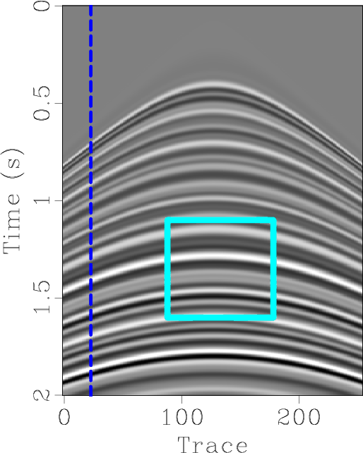
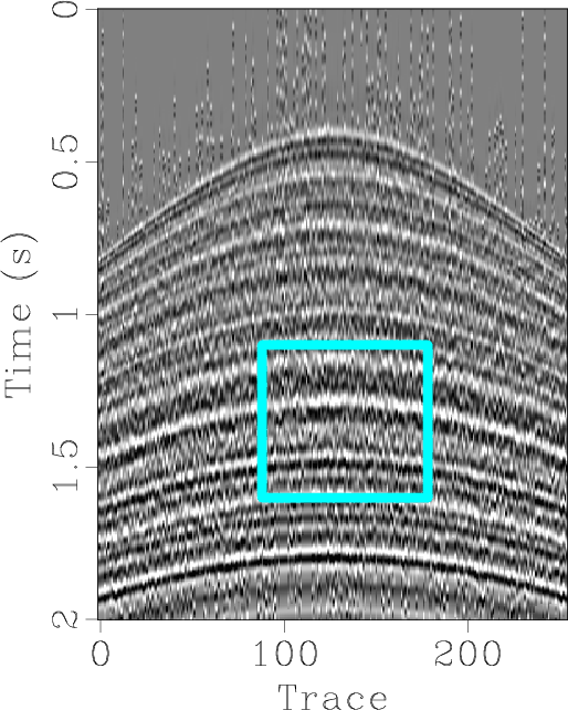
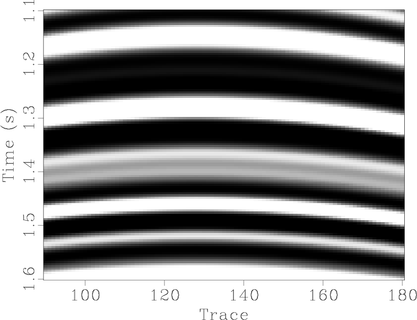
Figure 2. Simulated synthetic example. (a) Unblended data. (b) Blended data.

hdbor1-1,hdbst1-1,hdbft1-1,hdbfx1-1
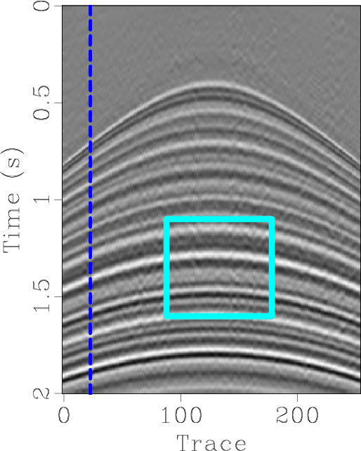
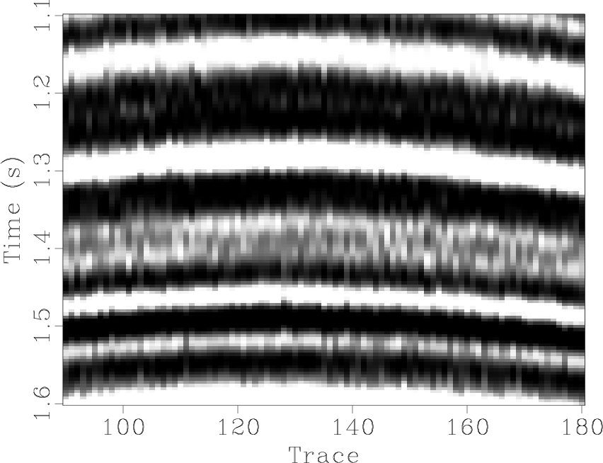
Figure 3. Simulated synthetic example. (a) Deblended data using the proposed approach. (b) Deblended data using seislet domain thresholding. (c) Deblended data using $f-k$ domain thresholding. (d) Deblended data using $f-x$ deconvolution.

heor1,hest1,heft1,hefx1
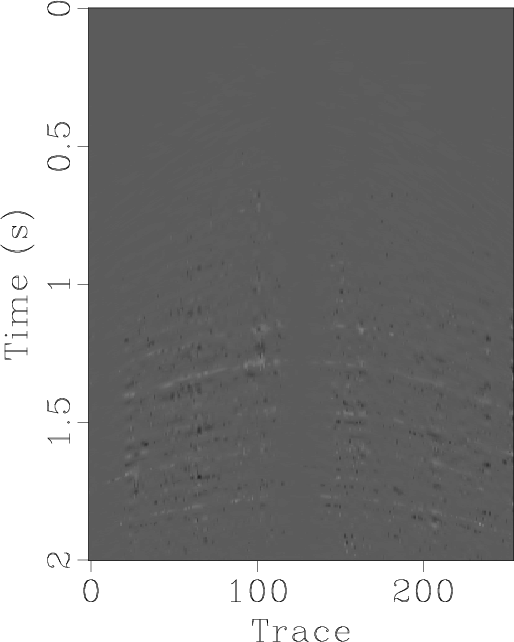
Figure 4. Simulated synthetic example. (a) Estimation error section using the proposed approach. (b) Estimation error section using seist domain thresholding. (c) Estimation error section using $f-k$ domain thresholding. (d) Estimation error section using $f-x$ deconvolution.

h1-z,hs-z,hdbor1-z-0,hdbst1-z-0,hdbft1-z,hdbfx1-z
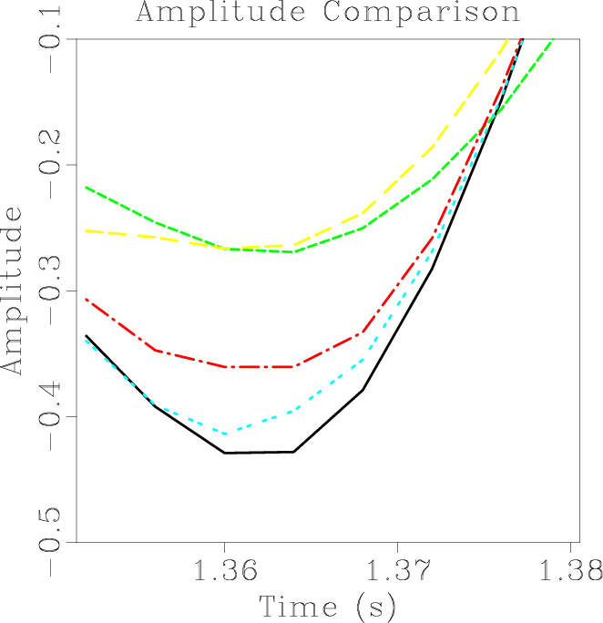
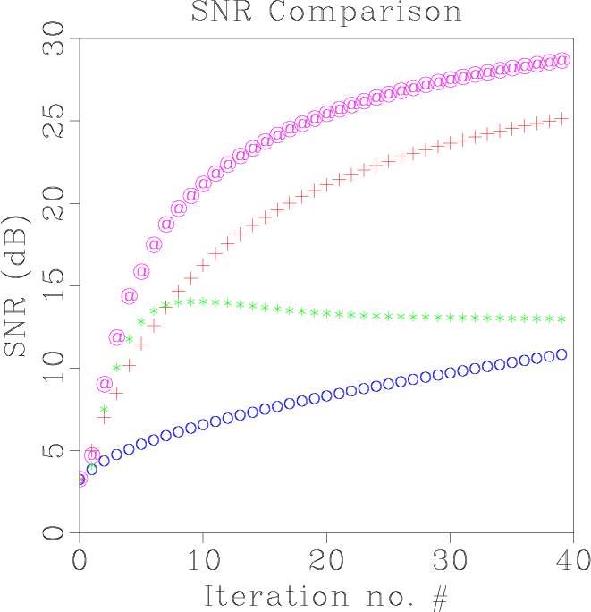
Figure 5. Zoomed section comparisons of the simulated synthetic example. (a) Unblended data. (b) Blended data. (c) Deblended data using the proposed approach. (d) Deblended data using seislet domain thresholding. (e) Deblended data using $f-k$ domain thresholding. (f) Deblended data using $f-x$ deconvolution.

hsnrsa,htc
Figure 6. (a) Comparison of signal-to-noise ratio of the simulated synthetic example. "@" refers to the proposed approach. "+" refers to seislet thresholding. "*" refers to $f-x$ deconvolution. "o" refers to $f-k$ thresholding. (b) Comparison of the amplitude between 1.35s and 1.38s of the 25th trace in the simulated synthetic data example. Black solid line denotes the unblended trace (true trace). Blue double dot line corresponds to the proposed approach. Red dot dash line corresponds to seislet thresholding. Green dash line corresponds to $f-k$ thresholding. Yellow long dash line corresponds to $f-x$ deconvolution.

Iterative deblending with multiple constraints based on shaping regularization