Appendix A: Review of local similarity

A common way to measure the similarity between two signals is to calculate the global correlation coefficient:

$\displaystyle \gamma=\frac{\displaystyle\sum_{i=1}^Na(i)b(i)}{\displaystyle\sqrt{\sum_{i=1}^Na^2(i)\sum_{i=1}^Nb^2(i)}},$ (14)

where $r$ is the global correlation coefficient, $N$ denotes the number of samples of the signals $\mathbf{a}$ and $\mathbf{b}$. In order to calculate the similarity between two signals locally, one can use the localized correlation coefficient:

$\displaystyle \gamma_m(t)=\frac{\displaystyle\sum_{i=t-m/2}^{t+m/2} a(i) b(i)}{...
...yle\sum_{i=t-m/2}^{t+m/2} a^2(i) \displaystyle\sum_{i=t-m/2}^{t+m/2} b^2(i) }},$ (15)

where $\gamma_m(t)$ denotes the local correlation coefficient, $m$ is the local window size.

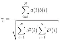
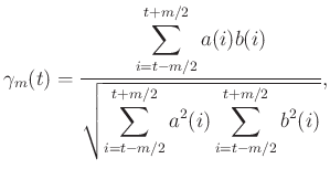
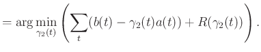
Fomel (2007a) designed an elegant way to calculate the local similarity:

$\displaystyle \gamma(t)$ $\displaystyle =\sqrt{\gamma_1(t)\gamma_2(t)},$ (16)
$\displaystyle \gamma_1(t)$ $\displaystyle =\arg\min_{\gamma_1(t)} \left(\sum_{t}(a(t)-\gamma_1(t)b(t)) + R(\gamma_1(t)) \right),$ (17)
$\displaystyle \gamma_2(t)$ $\displaystyle =\arg\min_{\gamma_2(t)} \left(\sum_{t}(b(t)-\gamma_2(t)a(t)) + R(\gamma_2(t)) \right).$ (18)

Equation 16 represents that the local similarity can be expressed as the product of two vectors that are the solutions of two minimization problems. $R$ is a regularization operator for constraining $\gamma_1$ and $\gamma_2$. $R$ can be chosen as a local triangular smoother to enforce the smoothness of vectors $\gamma_1$ and $\gamma_2$, and then equations 17 and 18 can be solved using the shaping regularization (Fomel, 2007b):

$\displaystyle \mathbf{\gamma}_1$ $\displaystyle = [\lambda_1^2\mathbf{I} + \mathcal{S}(\mathbf{B}^T\mathbf{B}-\lambda_1^2\mathbf{I})]^{-1}\mathcal{S}\mathbf{B}^T\mathbf{a},$ (19)
$\displaystyle \mathbf{\gamma}_2$ $\displaystyle = [\lambda_2^2\mathbf{I} + \mathcal{S}(\mathbf{A}^T\mathbf{A}-\lambda_2^2\mathbf{I})]^{-1}\mathcal{S}\mathbf{A}^T\mathbf{b},$ (20)

where $\mathbf{A}$ is a diagonal operator composed from the elements of $\mathbf{a}$: $\mathbf{A}=diag(\mathbf{a})$ and $\mathbf{B}$ is a diagonal operator composed from the elements of $\mathbf{b}$: $\mathbf{B}=diag(\mathbf{b})$. $\mathbf{\mathcal{S}}$ is a smoothing operator, and $\lambda_1$ and $\lambda_2$ are two parameters controlling the physical dimensionality and enabling fast convergence when inversion is implemented iteratively. These two parameters can be chosen as the least-squares norms of $\mathbf{A}$ and $\mathbf{B}$ (Fomel, 2007a). The local similarity algorithm can be used to calculate the local similarity of signal of any dimension. For 1D signals, the meanings of equations 19 and 20 are intuitive. For 2D or higher-dimensional signals, each signal is first reshaped into a 1D signal and then follows equations 19 and 20 to calculate the local similarity vector. The smoothing operator is applied to the 2D or multi-dimensional form of the original signal to enforce the smoothness in any dimension.


2020-04-11