 |
 |
 |
 | A fast butterfly algorithm for generalized Radon transforms |  |
![[pdf]](icons/pdf.png) |
Next: Field data
Up: Numerical examples
Previous: Synthetic data
Going back to the five steps of the butterfly algorithm, it is clear that the input data
 is only involved at the very first step. Besides, for every
  the operation connecting
and
the operation connecting
and
 amounts to a matrix-vector multiplication (see equation 23), which does not at all require the input data to be uniformly distributed (the same argument applies to the output data
 ). Therefore, our algorithm can be easily extended to handle the following problem:
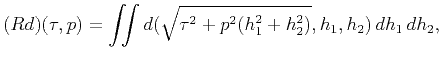 |
(28) |
where
 is a 3D function. All we need is to introduce a new variable for the absolute offset
 , and reorder the values
according to
, and reorder the values
according to  . Figure 12 shows such synthetic data sampled on
  ,
,
 . The output is obtained on
 ,
,  . The fast algorithm (Figure 13) runs in only 1.67 s for
  ,
,
 (here the range of
 is about 162), while the velocity scan (Figure 14) takes more than 125 s.

|
|---|
data-4
Figure 12. 3D synthetic CMP gather.
,
.
 s,
s,
 km.
km.
|
|---|
![[png]](icons/viewmag.png) ![[scons]](icons/configure.png)
|
|---|

|
|---|
fmod-4
Figure 13.
,
. Output of the fast butterfly algorithm applied to the synthetic data in Figure 12.
,
. CPU time: 1.67 s. Purple curve overlaid is the true slowness.
|
|---|
|
|
|---|

|
|---|
dimod-4
Figure 14.
,
. Output of the velocity scan applied to the synthetic data in Figure 12. CPU time: 125.54 s. Purple curve overlaid is the true slowness.
|
|---|
|
|
|---|
|
|
|
|
| A fast butterfly algorithm for generalized Radon transforms | |
|
Next: Field data
Up: Numerical examples
Previous: Synthetic data
2013-07-26