Velocity analysis using $AB$ semblance

Apendix A: Statistical analysis of semblance measures

In this appendix, I study the influence of noise on semblance measures. Let us assume that the signal $\mathbf{a}=a_1,a_2,\ldots,a_N$ is composed of random independent samples normally distributed with zero mean and $\sigma^2$ variance. In this case, the mathematical expectation for the semblance measure (3) is

$$E\left[\beta^2(\mathbf{a})\right] = \frac{\displaystyle E\left[\l... ...\right]} {\displaystyle N\,\sum_{i=1}^{N} E\left[a_i^2\right]} = \frac{1}{N}\;.$$ (9)

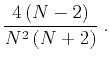
Correspondingly, the variance of the noise semblance is

$$V\left[\beta^2(\mathbf{a})\right] = \frac{\displaystyle E\left[\left(\sum_{i=1}^N a_i\right)^4\right]... ...sum_{i=1}^{N} \sum_{j \ne i} E\left[a_i^2\,a_j^2\right]\right)} - \frac{1}{N^2}$$

$$= \frac{3\,N\,\sigma^4 + 3\,(N^2-N)\,\sigma^4} {N^2\,\left[3\,N\,\s... ...4 + (N^2-N)\,\sigma^4\right]} - \frac{1}{N^2} = \frac{2\,(N-1)}{N^2\,(N+2)}\;.$$ (10)

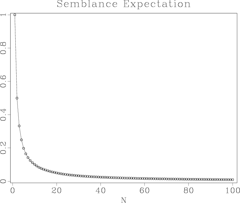
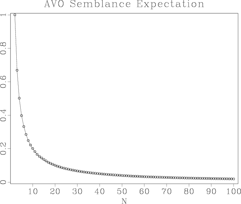
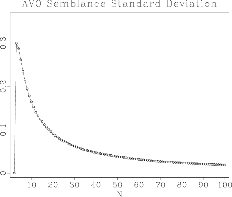
Equations (A-1) and (A-2) show that both the mathematical expectation and the standard deviation (the square root of variance) of the random noise semblance decrease at the rate of $1/N$ with the increase in the number of traces. To derive these equations, I make an assumption that the terms in the numerator and denominator are statistically independent. Rather than proving this assumption mathematically, I test it by numerical experiments with multiple random number realizations. Figure A-1 compares the theoretical prediction with experimental measurements from 10,000 random realizations.

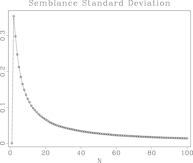
Applying similar analysis to the $AB$ semblance (7), we deduce that

$$E\left[\alpha^2(\mathbf{a})\right] = \frac{\displaystyle E\left[2\,\sum_{i=1}^{N} a_i\,\sum_{i=1}^N \p... ...]\, \left[\left(\sum_{i=1}^N \phi_i\right)^2 - N\,\sum_{i=1}^N \phi_i^2\right]}$$

$$= \frac{\displaystyle 2\,E\left[a_i^2\right]\,\left[\left(\sum_{i=1... ...um_{i=1}^N \phi_i\right)^2 - N\,\sum_{i=1}^N \phi_i^2\right]} = \frac{2}{N}\;.$$ (11)

and

$$V\left[\alpha^2(\mathbf{a})\right] = \frac{\displaystyle E\left[\left\{2\,\sum_{i=1}^{N} a_i\,\sum_{i=... ...um_{i=1}^N \phi_i\right)^2 - N\,\sum_{i=1}^N \phi_i^2\right]^2} - \frac{4}{N^2}$$

$$= \frac{\displaystyle 2\,\left[2\,\left(\sum_{i=1}^N \phi_i\right)^... ...um_{i=1}^N \phi_i\right)^2 - N\,\sum_{i=1}^N \phi_i^2\right]^2} - \frac{4}{N^2}$$

$$= \frac{4\,(N-2)}{N^2\,(N+2)}\;.$$ (12)

One can see that, in the case of the $AB$ semblance, the mathematical expectation and the standard deviation of the random noise semblance decrease at the rate of $2/N$ , twice higher than that for the conventional semblance. Figure A-2 compares the theoretical prediction with experimental measurements.

mean,vari
Figure 10. Mathematical expectation (a) and standard deviation (b) of random-noise semblance as functions of the number of traces $N$ . Solid lines are theoretical curves, circles are measurements from a numerical experiment.

amean,avari
Figure 11. Mathematical expectation (a) and standard deviation (b) of random-noise $AB$ semblance as a function of the number of traces $N$ . Solid lines are theoretical curves, circles are measurements from a numerical experiment.

Velocity analysis using $AB$ semblance