Seismic time-lapse image registration using amplitude-adjusted plane-wave destruction

Synthetic example

shiftd,tshifta,shifta,scalea,scaled,sunshift
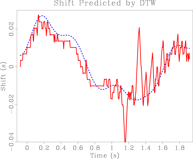
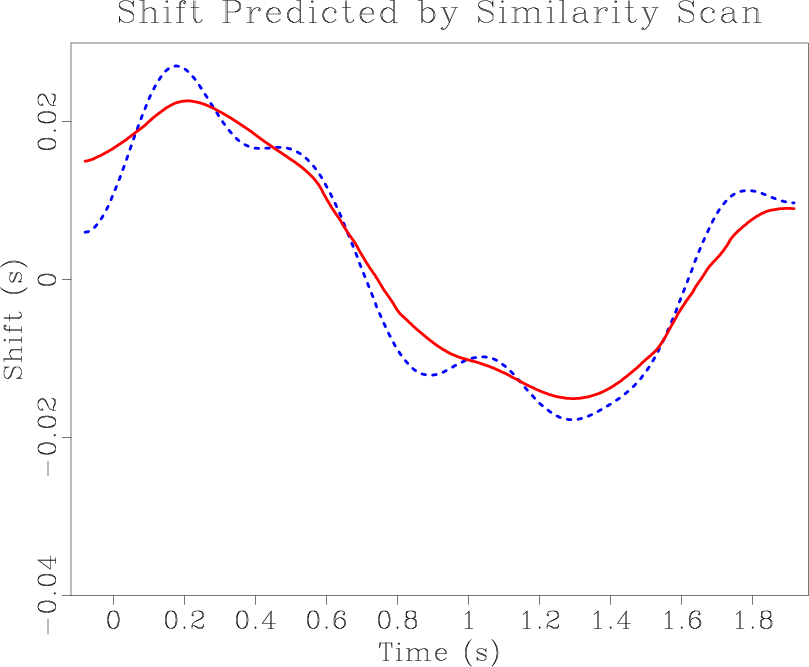
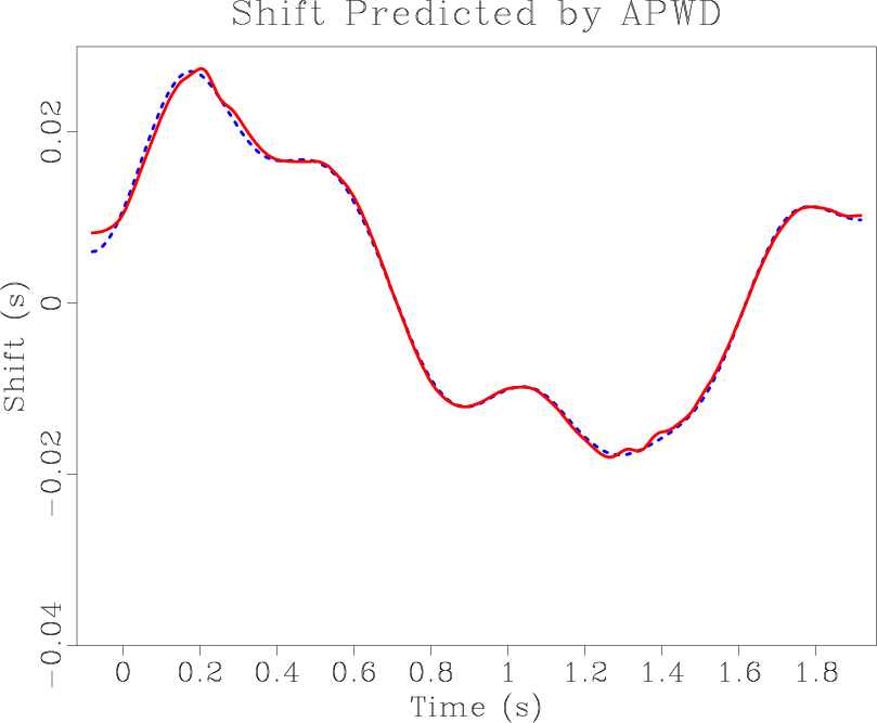
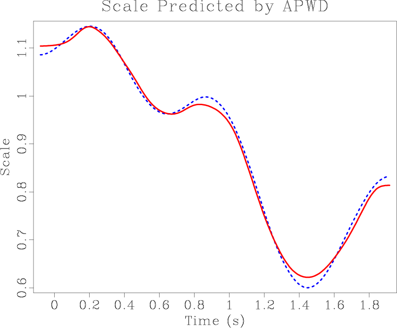
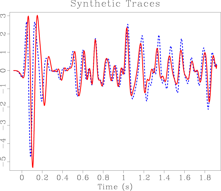
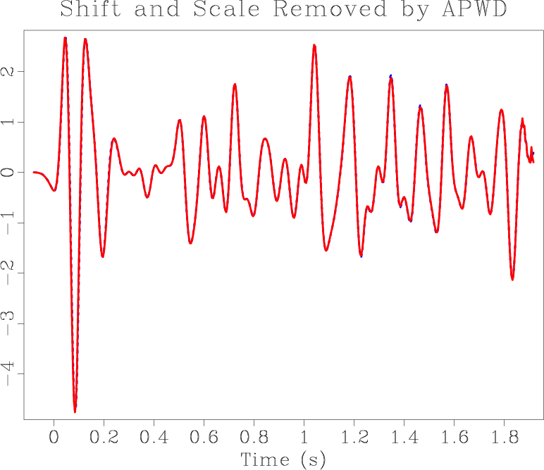
Figure 1. (a-c) Exact shift (dashed) and measured shift (solid) using: (a) dynamic time warping, (b) local similarity scanning, and (c) amplitude-adjusted plane-wave destruction. (d) Exact scaling function (solid) and measured scaling function using amplitude-adjusted plane-wave destruction (dashed), (e) synthetic base trace (dashed) and monitor trace (solid), and (f) synthetic base trace (dashed) and shifted and scaled monitor trace (solid) using shifting and scaling functions measured by amplitude-adjusted plane-wave destruction.

We first test the proposed algorithm by generating a random synthetic base trace, shifting function, and scaling function (Figure 1). The warping and scaling functions are applied to the base trace to create a synthetic monitor trace. We attempt to measure the shifting and scaling functions from the synthetic base and monitor traces using the proposed algorithm and compare the results with those from alternative algorithms.

We first apply the dynamic time warping algorithm (Sakoe and Chiba, 1978; Hale, 2013; Herrera and van der Baan, 2012). This algorithm is particularly effective when measuring large shifts, but it only computes integer shifts between samples on a pre-defined grid. In this synthetic example and many real examples from time-lapse monitoring, shifts are quite small and dynamic time warping is not always effective. Indeed, the shifting function measured with dynamic time warping does not effectively measure the small shifts in the synthetic trace and contains the unappealing ``stair-stepping" artifact due to the algorithm's inability to measure shifts outside of the predefined sampling grid (Figure 1a).

We then apply the local similarity scan (Fomel and Jin, 2009; Fomel, 2007) to measure the local shifting function. This algorithm scans through shifts, computing local similarity and picking the optimal warping path automatically. In our synthetic tests, this algorithm effectively measures the low frequency component of the synthetic shifting function, but fails to detect higher-frequency variations (Figure 1b).

Finally, we measure the shift using the proposed amplitude-adjusted plane-wave destruction algorithm. Compared to dynamic time-wapring and local similarity, plane-wave destruction proves to be particularly effective when measuring small, rapidly varying shifting functions. After only 5 iterations, the measured shifting function converges to the pre-defined synthetic shift (Figure 1c). We are also able to effectively measure the synthetic scaling function (Figure 1d). After applying the measured shifting and scaling functions to the synthetic monitor trace, the result is visually indistinguishable from the synthetic base trace (Figure 1f).

Seismic time-lapse image registration using amplitude-adjusted plane-wave destruction