Least-squares diffraction imaging using shaping regularization by anisotropic smoothing

Objective function

To solve for a seismic diffraction image $\mathbf {m}_d$ , we extend the approach developed by Merzlikin and Fomel (2016) to three dimensions:

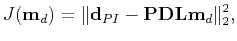$$J(\mathbf{m}_d) = \Vert\mathbf{d}_{PI} - \mathbf{PDL}\mathbf{m}_d\Vert _{2}^{2},$$ (1)

where $J(\mathbf{m}_d)$ is the objective function, $\mathbf {d}_{PI} = \mathbf {PDd}$ and $\mathbf {d}$ is ``observed'' data. Here, forward modeling corresponds to the chain of operators: three-dimensional path-summation integral filter $\mathbf{P}$ (Merzlikin and Fomel, 2015,2017), azimuthal plane wave destruction (AzPWD) filter $\mathbf {D}$ (Merzlikin et al., 2017b,2016) and three-dimensional Kirchhoff modeling $\mathbf{L}$ . The path-summation integral filter $\mathbf{P}$ can be treated as the probability of a diffraction at a certain location. Azimuthal plane wave destruction filter $\mathbf {D}$ removes reflected energy perpendicular to the edges. Therefore, AzPWD emphasizes edge diffraction signature, which when measured in the direction perpendicular to the edge exhibits a hyperbolic moveout and kinematically behaves as a reflection when observed along the edge. AzPWD application is the key distinction from the 2D version of the workflow (Merzlikin and Fomel, 2016), in which plane-wave destruction filter (PWD) (Fomel, 2002) is applied along the time-distance plane (Fomel et al., 2007; Merzlikin et al., 2018). After weighting the data $\mathbf {d}_{PI} = \mathbf {PDd}$ by path-summation integral $\mathbf{P}$ and AzPWD filter $\mathbf {D}$ , model fitting is constrained to most probable diffraction locations.

Least-squares diffraction imaging using shaping regularization by anisotropic smoothing