|
|
|
|
Least-squares diffraction imaging using shaping regularization by anisotropic smoothing |
The second field data example comes from the Cooper Basin onshore Western Australia.
The dataset corresponds to stacked (with
![]() m
bin size) preprocessed data acquired as a 3D land seismic survey
with fully azimuthal distribution of offsets and a far offset of
m
bin size) preprocessed data acquired as a 3D land seismic survey
with fully azimuthal distribution of offsets and a far offset of
![]() m
.
Preprocessing sequence includes noise attenuation, near-surface static corrections, despike, surface-consistent deconvolution,
Q-compensation whitening and time-variant filter applied after stacking.
The target horizon slice picked by the interpreter and used
for the performance evaluation of the method corresponds to the interface between tight-gas sand and coals (Tyiasning et al., 2016).
The depth of the interface is approximately
m
.
Preprocessing sequence includes noise attenuation, near-surface static corrections, despike, surface-consistent deconvolution,
Q-compensation whitening and time-variant filter applied after stacking.
The target horizon slice picked by the interpreter and used
for the performance evaluation of the method corresponds to the interface between tight-gas sand and coals (Tyiasning et al., 2016).
The depth of the interface is approximately
![]() m
. Structural complexity of the overburden can be characterized as high.
Detailed geological description of the area as well as the comparison of diffraction imaging results to discontinuity-type attributes is given by
Tyiasning et al. (2016).
Here, we apply the developed approach to the dataset.
Prestack time migration velocity is used for both full-wavefield migration and the proposed inversion approach for edge diffraction imaging.
m
. Structural complexity of the overburden can be characterized as high.
Detailed geological description of the area as well as the comparison of diffraction imaging results to discontinuity-type attributes is given by
Tyiasning et al. (2016).
Here, we apply the developed approach to the dataset.
Prestack time migration velocity is used for both full-wavefield migration and the proposed inversion approach for edge diffraction imaging.
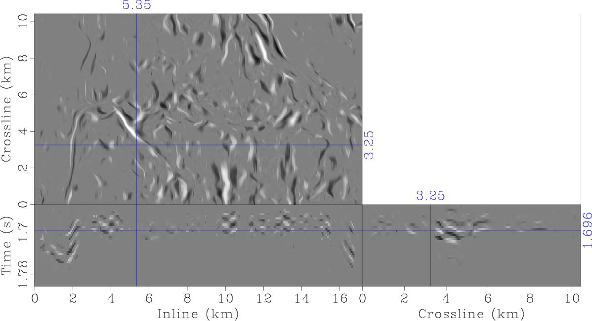
Figure 11 shows a stacked volume of the dataset. We focus on the window around the target horizon, which on average corresponds to
![]() s
TWTT.
Figure 12a shows conventional image of the target horizon slice generated with 3D post-stack time Kirchhoff migration.
We then apply reflection removal
procedure to the stack (Figure 11), migrate it, and generate the image shown in Figure 12b. Smaller scale features become highlighted, e.g.,
faults between
s
TWTT.
Figure 12a shows conventional image of the target horizon slice generated with 3D post-stack time Kirchhoff migration.
We then apply reflection removal
procedure to the stack (Figure 11), migrate it, and generate the image shown in Figure 12b. Smaller scale features become highlighted, e.g.,
faults between
![]() km
inlines and
km
inlines and
![]() km
crosslines. Acquisition footprint is noticeable on both of the images (Figure 12) and corresponds
to the low-amplitude events aligned in a grid-like fashion (easy to notice between inlines
km
crosslines. Acquisition footprint is noticeable on both of the images (Figure 12) and corresponds
to the low-amplitude events aligned in a grid-like fashion (easy to notice between inlines
![]() km
and crosslines
km
and crosslines
![]() km
).
We apply the developed workflow to further highlight and denoise diffractions.
km
).
We apply the developed workflow to further highlight and denoise diffractions.

|
|---|
|
stack-barrolka
Figure 11. 3D sesimic dataset from the Cooper Basin onshore Western Australia: stacked volume. |
|
|


|
|---|
|
mig3-ts,xspr-mig3-ts
Figure 12. Target horizon slice (the interface between tight-gas sand and coals picked by the interpreter ( |
|
|
First, we generate the data to be fit by the inversion - the stack weighted by a path-summation integral after reflection elimination (Figure 13a).
We run twenty outer and two inner iterations and use ![]() ,
,
![]() ,
, ![]() and
and ![]() .
As in the previous data example we use a low number of internal iterations to avoid noise fitting in general and footprint in particular. The inversion result along the target horizon is shown
in Figure 13b.
3D cubes of the migrated stack, the
migrated stack after reflection elimination and the inversion result are shown in Figures 14, 15 and 16.
Edges masked by the specular energy on the full-wavefield image (Figure 14), are highlighted on the image after
reflection elimination (Figure 15). At the same time,
edge diffractions produced by the inversion (Figure 16) appear to be clearer and have higher signal-to-noise ratio.
.
As in the previous data example we use a low number of internal iterations to avoid noise fitting in general and footprint in particular. The inversion result along the target horizon is shown
in Figure 13b.
3D cubes of the migrated stack, the
migrated stack after reflection elimination and the inversion result are shown in Figures 14, 15 and 16.
Edges masked by the specular energy on the full-wavefield image (Figure 14), are highlighted on the image after
reflection elimination (Figure 15). At the same time,
edge diffractions produced by the inversion (Figure 16) appear to be clearer and have higher signal-to-noise ratio.
Further, we apply Kirchhoff modeling to the inversion result (Figures 13b and 16), restore diffractions (Figure 17), and subtract the result from the stack after reflection elimination (Figure 18). The result of subtraction shown in Figure 19 can be treated as noise eliminated during the inversion. Signal and noise orthogonalization (Chen and Fomel, 2015) is applied to account for aperture difference between observed and restored diffractions (for instance, often only a single diffraction flank can be observed in the data leading to spuriously high difference or the ``noise estimate") and to bring back some of the energy accidentally leaked to the noise domain.
The acquisition footprint evident in Figure 19 suggests the
high performance of the method. Improvement can be noticed between
![]() km
inlines and
km
inlines and
![]() km
crosslines associated
with the extraction of small-scale discontinuities. Compare the inversion result Figure 13b
and the result of migration shown in Figure 12b. Same subtle events are located at crossline
km
crosslines associated
with the extraction of small-scale discontinuities. Compare the inversion result Figure 13b
and the result of migration shown in Figure 12b. Same subtle events are located at crossline
![]() km
between inlines
km
between inlines
![]() km
(Figures 17 and 18) and have a clear hyperbolic shape
(Figure 17), which appears when edge diffractions are observed perpendicular to edges.
Good restoration quality can also be inferred from the ``circular" structure
between
km
(Figures 17 and 18) and have a clear hyperbolic shape
(Figure 17), which appears when edge diffractions are observed perpendicular to edges.
Good restoration quality can also be inferred from the ``circular" structure
between
![]() km
inlines and
km
inlines and
![]() km
crosslines. Both of these areas
have high similarity between the initial diffraction stack (Figure 18) and the stack with diffractions ``restored" and denoised by inversion (Figure 17)
leading to low amplitudes in the difference section (Figure 19) primarily associated with noise. These features also follow ``frowning"-focusing-``smiling"
behaviour under migration velocity perturbation supporting their diffraction nature in the plane perpendicular to the edge.
km
crosslines. Both of these areas
have high similarity between the initial diffraction stack (Figure 18) and the stack with diffractions ``restored" and denoised by inversion (Figure 17)
leading to low amplitudes in the difference section (Figure 19) primarily associated with noise. These features also follow ``frowning"-focusing-``smiling"
behaviour under migration velocity perturbation supporting their diffraction nature in the plane perpendicular to the edge.


|
|---|
|
linpi-data-ts,modl-test-ts
Figure 13. Target horizon slice (the interface between tight-gas sand and coals picked by the interpreter ( |
|
|

|
|---|
|
mig3-barrolka
Figure 14. 3D post-stack Kirchhoff migration of the stack shown in Figure 11. |
|
|

|
|---|
|
xspr-mig3-barrolka
Figure 15. 3D post-stack Kirchhoff migration of the stack (Figure 11) after reflection elimination and edge diffraction extraction with AzPWD. Subsurface discontinuities appear to be highlighted in comparison to Figure 14, in which they are masked by specular energy. At the same time, diffraction image still has some noise present. |
|
|
|
|---|
|
modl-test
Figure 16. Inversion result. Edge diffractions are both highlighted and denoised (compare with Figure 15). |
|
|

|
|---|
|
diffractions-ortho-barrolka
Figure 17. Kirchhoff modeling of diffractivity from Figure 16. ``Clean'' diffraction signatures are recovered: notice hyperbolic shapes when edge diffractions are observed perpendicular to edges. |
|
|

|
|---|
|
xspr-notmig-barrolka
Figure 18. Stack with reflections removed. The majority of reflections is removed, some hyperbolic signatures can be seen (compare with Figures 11 and 17). Reflection remainders and noise including acquisition footprint are apparent (compare with Figure 17). |
|
|

|
|---|
|
noise-ortho-barrolka
Figure 19. Difference between Figures 17 and 18 is predominated by noise and thus supports the validity of denoised edge diffractions (Figure 17). |
|
|
Some features are lost in the area between
![]() km
inlines and
km
inlines and
![]() km
crosslines. Event between inlines
km
crosslines. Event between inlines
![]() km
and crosslines
km
and crosslines
![]() km
is not predicted (Figure 19).
High magnitude events observed between inlines
km
is not predicted (Figure 19).
High magnitude events observed between inlines
![]() km
at crossline
km
at crossline
![]() km
and between crosslines
km
and between crosslines
![]() km
at inline
km
at inline
![]() km
(Figure 16 and 17)
can be associated with reflections leaked to the diffraction image domain
or can actually be edge diffractions observed in the plane not perpendicular to the edge and thus having elongated signature.
The event located at crossline
km
(Figure 16 and 17)
can be associated with reflections leaked to the diffraction image domain
or can actually be edge diffractions observed in the plane not perpendicular to the edge and thus having elongated signature.
The event located at crossline
![]() km
between inlines
km
between inlines
![]() km
inversion interprets as a reflection and removes it
from the diffraction imaging result (Figure 16 and 17).
High difference values following the channel in the difference cube (Figure 19)
can also be associated with the reflection remainders removed from the diffraction image domain.
km
inversion interprets as a reflection and removes it
from the diffraction imaging result (Figure 16 and 17).
High difference values following the channel in the difference cube (Figure 19)
can also be associated with the reflection remainders removed from the diffraction image domain.
It should be mentioned that the target horizon has a highly oscillating pattern including a high magnitude drop
in the left part of the cube (inlines
![]() km
) making dip estimation for ``ideal" reflection-diffraction separation simultaneously for the whole area challenging. More careful
dip estimation possibly with different parameters in different regions of the dataset should further improve the result. Inversion parameters can definitely be tweaked
to improve the results but even with these trial values the majority of the edges including some subtle features
(e.g., events at crossline
km
) making dip estimation for ``ideal" reflection-diffraction separation simultaneously for the whole area challenging. More careful
dip estimation possibly with different parameters in different regions of the dataset should further improve the result. Inversion parameters can definitely be tweaked
to improve the results but even with these trial values the majority of the edges including some subtle features
(e.g., events at crossline
![]() km
between inlines
km
between inlines
![]() km
(Figure 16)) hardly noticeable on
the migrated stack after reflection elimination (Figure 15)
has been extracted and highlighted.
km
(Figure 16)) hardly noticeable on
the migrated stack after reflection elimination (Figure 15)
has been extracted and highlighted.
|
|
|
|
Least-squares diffraction imaging using shaping regularization by anisotropic smoothing |