Traveltime approximations for transversely isotropic media with an inhomogeneous background

The vertical direction

The vertical direction in the conventional seismic experiment is critical as the depth mistie (or vertical velocity) and the NMO velocity are typically measured with respect to the vertical direction regardless of the tilt in the symmetry angle. 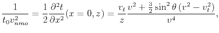Specifically, the vertical velocity is extracted from the well check shots (typically vertical) and the moveout velocity given by the second derivative of traveltime with respect to phase angle, is measured in the vertical direction ($x=0$). Setting $x=0$ in equation 9, and considering the two-way traveltime, $t=2\tau$, yields the following relation for the traveltime in the vertical direction:

$$t(x=0,z)=2 \frac{z}{v_{t}} \left(1-\frac{1}{2} \sin^{2}\theta \left(1-\frac{v_{t}^{2}}{v^{2}} \right) \right),$$ (16)

which includes terms related to the symmetry-axis direction. From Figure 2 we can see how well this approximation predicted the vertical traveltime. This equation is convenient to use along with well information to predict the velocities along the symmetry axis. Actually, for $\eta \ne 0$ (anelliptic TI media), applying Pade approximations (Bender and Orszag, 1978) to the $\eta$ and $\sin\theta$ expansions, yields the following relation for traveltime in the vertical direction:

$$t(x=0,z)=2 \frac{z}{v_{t}} \frac{v^{2}}{v^{2} +\frac{1}{2} \sin^{2}\theta \left(v^{2}-v_{t}^{2} \right)}.$$ (17)

Note that this equation is independent of $\eta$, which implies that for small tilt angles, $\eta$ has practically no influence on the vertical traveltime. This fact helps us better construct the background elliptical anisotropy, as $\eta$ has little influence on this process for small tilt angles. Combine the above equations with those related to the NMO (stacking) velocity in the vertical direction:

$$\frac{1}{t_0 v_{nmo}^{2}} = \frac{1}{2} \frac{\partial^{2} t}{\pa... ... \frac{v^{2} +\frac{3}{2} \sin^{2}\theta \left(v^{2}-v_{t}^{2} \right)}{v^{4}},$$ (18)

where $t_0$ is given by equation 16. If we use Shanks transform again for higher-order accuracy, such an NMO velocity equation has the following form:

$$\frac{1}{t_0 v_{nmo}^{2}} = \frac{z}{v_{t}} \frac{8 v_t^2 v^4-2 \... ...heta}{z^2 \left(v^2 \left(\sin ^2\theta+2\right)-v_t^2 \sin ^2\theta\right)^3},$$ (19)

where $t_0$ is given by equation 18. Again, these equations are independent of $\eta$. The combination of equations 16 and 18 or equations 17 and 19 for a known tilt direction can be used to estimate the velocity along the symmetry axis as well as $\delta$ ( $=\frac{v^{2}-v_{t}^{2}}{2 v_{t}^{2}}$). Specifically, the above formulations provide a mechanism to evaluate the symmetry-direction (anisotropy) parameters from measurements obtained using the conventional seismic experiment, vertical and stacking velocities.

Focusing on the performance of approximation 8 for small offsets allows us to predict the accuracy of equations 16 and 18 as they are derived from equation 8. Figure 4 repeats the example of Figure 2 with a tilt of $5^{o}$ (a), $10^{o}$ (b), and $20^{o}$ (c), and a focus on small offsets (near vertical). Of course, errors increase with the increase in the tilt angle as all approximations are for small tilt angles from vertical. Though the vertical direction error in the case of the new equations is higher, the slope of the error is almost zero indicating that the new equation should provide a good estimation of the NMO velocity (extracted from the second derivative of traveltime with respect to offset). This feature is critical since the errors associated with the other approximations (i.e. Sena (1991)) for the NMO representation are large. This also explains the higher accuracy of the new equations at higher offsets as the error gradient is small. It is also clear from Figure 4 that using Pade approximations to predict the higher-order terms of the expansion in $\theta$ did not increase the accuracy much (the difference between solid and dashed black curves). This is also observed for anelliptic TI as we will see next.

verticaleta0
Figure 4. The relative traveltime error as a function of offset (near zero offset) for an elliptical anisotropic model with $v$=2 km/s, $\delta =\epsilon =0.2$, $\theta =20^{0}$, and a reflector depth $z$=2 km for the new expansion (equation 8) in $\theta$ (dashed black curve), the new expansion with Pade approximation in $\theta$ (solid black curve), and for the Sena approximation (solid gray curve). The plots correspond to (a) a 5 degree tilt, (b) a 10 degree tilt, and (c) a 20 degree tilt.

For anelliptic TI media with $\delta =0.1$ and $\epsilon =0.2$, I obtain similar results. Figure 5 shows the traveltime error over a limited offset for three symmetry tilt angles: (a) $5^{o}$, (b) $10^{o}$, and (c) $20^{o}$. Again, the accuracy of the new equations is apparent in the slope of the error near zero offset, implying that the NMO velocity representation is highly accurate. The errors in the vertical velocity, though, are the largest for the new equations. However, the vertical velocity genrally has less influence than the NMO velocity on time processing objectives.

vertical
Figure 5. The relative traveltime error as a function of offset (near zero offset) for a TI model with $v$=2 km/s, $\delta =0.1$, $\epsilon =0.2$, $\theta =20^{0}$, and a reflector depth $z$=2 km for the new expansion (equation 8) in $\theta$ (dashed black curve), the new expansion with Pade approximation in $\theta$ (solid black curve), and for the Sena approximation (solid gray curve). The plots correspond to (a) a 5 degree tilt, (b) a 10 degree tilt, and (c) a 20 degree tilt.

Finally, for a TI medium with $\delta =0.0$ and $\epsilon =0.2$ (Figure 6) we observe similar behavior with smaller overall relative errors compared to Figures 4 and 5. As $\delta$ decreases, the anisotropy influence near the vertical direction decreases, and the effect of the tilt is less pronounced. However, when the tilt is larger, Figure 6c, the errors are large and comparable to those in Figures 4c and 5c as the influence of $\eta$ starts to appear.

verticaleta2
Figure 6. The traveltime error as a function of offset (near zero offset) for a TI anisotropic model with $v$=2 km/s, $\delta =0.0$, $\epsilon =0.2$, $\theta =20^{0}$, and a reflector depth $z$=2 km for the new expansion (equation 8) in $\theta$ (dashed black curve), the new expansion with Pade approximation in $\theta$ (solid black curve), and for the Sina approximation (solid gray curve). The plots correspond to (a) a 5 degree tilt, (b) a 10 degree tilt, and (c) a 20 degree tilt.

In the above examples we note that despite the inferior accuracy of equations 16 and 18 in representing the vertical traveltime, with relative errors that could reach 0.3 percent for the 20 degree tilt case, it has superior qualities in predicting the NMO velocity. This phenomenon is explained by the fact that the new equations are expansions with respect to tilt angle, while the other equations are expansions with respect to offset (or anisotropy parameters), thus they provide better accuracy near zero offset. In contrast, the new equations tend to be more offset independent and better represent the moveout over larger offsets.

Traveltime approximations for transversely isotropic media with an inhomogeneous background