|
|
|
|
Wavefield extrapolation in pseudodepth domain |
The ![]() domain wave equations in the previous section are derived for 3D models. For simplicity, the examples in this paper is for D models.
Since the change in the vertical axis acts on a single vertical velocity profile at a time, the conclusions in this section can be extended to 3D case.
To test the accuracy of the
domain wave equations in the previous section are derived for 3D models. For simplicity, the examples in this paper is for D models.
Since the change in the vertical axis acts on a single vertical velocity profile at a time, the conclusions in this section can be extended to 3D case.
To test the accuracy of the ![]() domain wavefield extrapolation, we look at impulse responses of the
domain wavefield extrapolation, we look at impulse responses of the ![]() domain migration operators and compare them
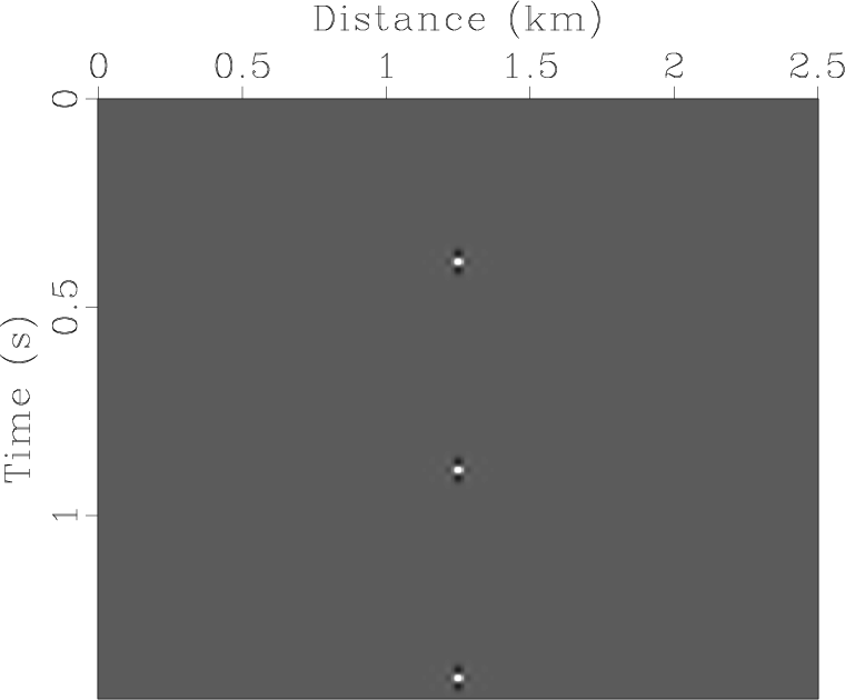
with those obtained from the Cartesian domain extrapolations. A synthetic zero-offset section with three spikes are illustrated in Figure 4.
Migration images obtained from this section are superpositions of the Green's functions due to a point source located at the center on the surface.
domain migration operators and compare them
with those obtained from the Cartesian domain extrapolations. A synthetic zero-offset section with three spikes are illustrated in Figure 4.
Migration images obtained from this section are superpositions of the Green's functions due to a point source located at the center on the surface.
|
spike
Figure 4. Zero-offset section with three impulse events equally spaced in time. The source has peak frequency of |
|
|---|---|
|
|
Our first example is a lens velocity model, shown in Figure 5(a).
The background velocity is
![]() and contains a negative anomaly of
and contains a negative anomaly of
![]() . We use the same velocity to obtain vertical time
. We use the same velocity to obtain vertical time ![]() , i.e.
, i.e. ![]() in Equation 2. The
in Equation 2. The ![]() mesh is overlaid on the velocity model, a prominent ``pull-down'' near the bottom of the model is due to the slow velocity lens. By the same analogy, a ``push-up'' will appear in the
mesh is overlaid on the velocity model, a prominent ``pull-down'' near the bottom of the model is due to the slow velocity lens. By the same analogy, a ``push-up'' will appear in the ![]() domain beneath a positive velocity anomaly, for example a salt body. By applying the change of variable in Equation 2, the velocity is interpolated to the
domain beneath a positive velocity anomaly, for example a salt body. By applying the change of variable in Equation 2, the velocity is interpolated to the ![]() domain and plotted in Figure 5(b).
The
domain and plotted in Figure 5(b).
The ![]() axis is discretized by
axis is discretized by ![]() samples to speedup extrapolation and honor the aliasing condition.
The zero-offset section in Figure 4 is migrated using Equation 10 by extrapolating backward in time and applying zero-time imaging condition. The resulting image is shown in Figure 5(c).
In the
samples to speedup extrapolation and honor the aliasing condition.
The zero-offset section in Figure 4 is migrated using Equation 10 by extrapolating backward in time and applying zero-time imaging condition. The resulting image is shown in Figure 5(c).
In the ![]() domain, the extrapolation is done by solving Equation 15. Following the same imaging condition, the migrated image is shown in Figure 5(d).
This image is then interpolated back to the Cartesian domain using equation 4, and compared with Figure 5(c).
The error shown in Figure 5(f)
is due to the linear interpolation between Cartesian and
domain, the extrapolation is done by solving Equation 15. Following the same imaging condition, the migrated image is shown in Figure 5(d).
This image is then interpolated back to the Cartesian domain using equation 4, and compared with Figure 5(c).
The error shown in Figure 5(f)
is due to the linear interpolation between Cartesian and ![]() meshes, and it is relatively small.
meshes, and it is relatively small.


|
|---|
|
lengC,lengT,leniC,leniT,leniB,leniE
Figure 5. A lens velocity model in (a) Cartesian and (b) |
|
|
The next examples demonstrate extrapolation in complex models.
In Figure 6(a), we show a section of the isotropic Marmousi velocity model. Since the vertical time derived from this velocity has very ragged curvatures that may pose stability difficulties for the ![]() domain extrapolation, in Equation 2 we use instead a smoothed version of the Marmousi velocity as
domain extrapolation, in Equation 2 we use instead a smoothed version of the Marmousi velocity as ![]() to compute
to compute ![]() . Interpolation of the Marmousi velocity on to the
. Interpolation of the Marmousi velocity on to the ![]() mesh is shown in Figure 6(b).
Impulse responses are obtained by solving Equations 10 (Figure 6(c)) and 15 (Figure 6(d)).
The error is plotted in Figure 6(f) and it is relatively small.
mesh is shown in Figure 6(b).
Impulse responses are obtained by solving Equations 10 (Figure 6(c)) and 15 (Figure 6(d)).
The error is plotted in Figure 6(f) and it is relatively small.


|
|---|
|
margC,margT,mariC,mariT,mariB,mariE
Figure 6. A portion of the Marmousi velocity in (a) Cartesian and (b) |
|
|
Extrapolation of anisotropic wavefields in the ![]() coordinates system is also feasible. The propagation of quasi-acoustic P waves is characterized by three parameters: vertical
coordinates system is also feasible. The propagation of quasi-acoustic P waves is characterized by three parameters: vertical ![]() -wave velocity
-wave velocity ![]() , NMO velocity
, NMO velocity ![]() and the anellipticity
and the anellipticity ![]() .
For example, the anisotropic parameters of the SEG/Hess model are shown in Figures 7(a) to 7(c).
.
For example, the anisotropic parameters of the SEG/Hess model are shown in Figures 7(a) to 7(c).


|
|---|
|
hesm1,hesm2,hesm3
Figure 7. A portion of the SEG/Hess anisotropic velocity model. (a) Vertical velocity (b) NMO velocity (c) |
|
|
Similar to isotropic complex models, to alleviate the distortion of the ![]() mesh due to the strong velocity variation of the salt body, the
mesh due to the strong velocity variation of the salt body, the ![]() mesh is constructed using a smooth background velocity
mesh is constructed using a smooth background velocity ![]() .
The resulting
.
The resulting ![]() coordinate system is overlaid on vertical velocities in the Cartesian and
coordinate system is overlaid on vertical velocities in the Cartesian and ![]() domains, shown in Figure 8(a) and 8(b).
The Cartesian domain impulse response is computed from Equation 20, Figure 8(c) shows the horizontal stress field
domains, shown in Figure 8(a) and 8(b).
The Cartesian domain impulse response is computed from Equation 20, Figure 8(c) shows the horizontal stress field ![]() .
In the
.
In the ![]() domain, the impulse response is obtained from equation 21, and the resulting
domain, the impulse response is obtained from equation 21, and the resulting ![]() field is shown in Figure 8(d).
As expected, the wavefield beneath the salt is ``pushed up'' due to positive velocity anomaly at salt dome.
The error in the migration image obtained in
field is shown in Figure 8(d).
As expected, the wavefield beneath the salt is ``pushed up'' due to positive velocity anomaly at salt dome.
The error in the migration image obtained in ![]() domain is plotted in Figure 8(f).
domain is plotted in Figure 8(f).


|
|---|
|
hesgC,hesgT,hesiC,hesiT,hesiB,hesiE
Figure 8. The vertical velocity in (a) the Cartesian and (b) the |
|
|
Table 1 summarizes the numerical cost of wavefield extrapolation in Cartesian and ![]() domains. For isotropic extrapolations, elapsed time is shorter in
domains. For isotropic extrapolations, elapsed time is shorter in ![]() domain than in Cartesian domain, the percentage cut is close to the reduction of vertical sampling of the wavefield. For anisotropic extrapolations, the efficiency improvement is less significant, due to the increased number of derivatives on the right-hand side of equations 21 as compared to Cartesian extrapolator 20.
domain than in Cartesian domain, the percentage cut is close to the reduction of vertical sampling of the wavefield. For anisotropic extrapolations, the efficiency improvement is less significant, due to the increased number of derivatives on the right-hand side of equations 21 as compared to Cartesian extrapolator 20.
| Model | reduction | speedup | ||||
| Lens (Figure 5(a)) | 401 | 251 | 37.5% | 18 | 12 | 33.3% |
| Marmousi (Figure 6(a)) | 751 | 501 | 33.3% | 277 | 193 | 30.3% |
| SEG/Hess (Figure 8(a)) | 601 | 501 | 16.6% | 102 | 98 | 3.9% |
In addition to the reduced computational cost, ![]() anisotropic extrapolation also features attenuated shear wave artifacts. Figure 9 shows the impulse responses using a homogeneous anisotropic velocity model. The shear wave artifact is significant in the Cartesian domain, shown on the left.
In the
anisotropic extrapolation also features attenuated shear wave artifacts. Figure 9 shows the impulse responses using a homogeneous anisotropic velocity model. The shear wave artifact is significant in the Cartesian domain, shown on the left.
In the ![]() domain, the artifact is attenuated with the coarser vertical sampling, as shown on the right. Coarser sampling enhance numerical dispersion of the shear wave, which tends to spread the energy across the domain, thus attenuates the shear wave artifact.
domain, the artifact is attenuated with the coarser vertical sampling, as shown on the right. Coarser sampling enhance numerical dispersion of the shear wave, which tends to spread the energy across the domain, thus attenuates the shear wave artifact.


|
|---|
|
arteC,arteZ,arteT
Figure 9. Anisotropic impulse response obtained in Cartesian (Left) and |
|
|
|
|
|
|
Wavefield extrapolation in pseudodepth domain |