|
|
|
|
Wavefield extrapolation in pseudodepth domain |
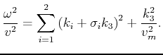
A geometrical description of the ![]() domain isotropic wavefield can be achieved by looking at its eikonal. A dispersion relation associated with the
domain isotropic wavefield can be achieved by looking at its eikonal. A dispersion relation associated with the ![]() domain wave equation 15 is obtained by taking Fourier transform of this equation in space and time, specifically, do the substitution
domain wave equation 15 is obtained by taking Fourier transform of this equation in space and time, specifically, do the substitution
![]() and
and
![]() , the result is
, the result is
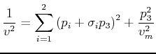
We then relate slowness vector
![]() with wavenumber vector
with wavenumber vector
![]() by
by
![]() , thus the
, thus the ![]() domain isotropic eikonal equation is
domain isotropic eikonal equation is
|
|
|
|
Wavefield extrapolation in pseudodepth domain |