|
|
|
|
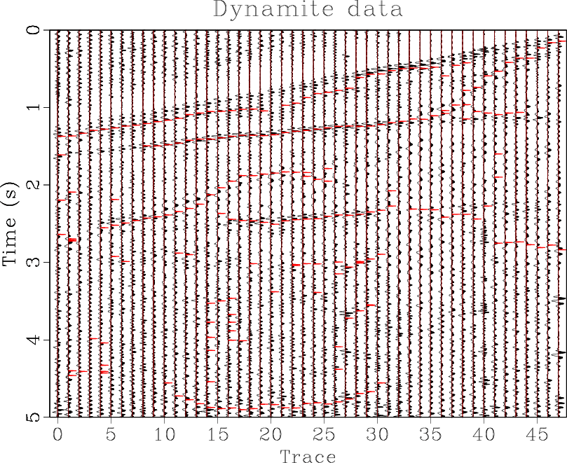
Automatic traveltime picking using the instantaneous traveltime |
In this application, we effectively applied an automatic picking tool to raw two-dimensional seismic data without imposing any consistency requirements over offset. Our objective was to measure the capability of this attribute in mapping reflections. The figure shows that the instantaneous traveltime attribute misses many of the first breaks due to the complexity of the waveforms of the early arrivals. The proposed method is therefore not suitable for picking first breaks, although the instantaneous traveltime can be used for automatic first-break picking, if applied appropriately (Saragiotis and Alkhalifah, 2012). Nevertheless, the first reflection is clearly well picked at most traces as is the 1.5 km/s refraction. The second reflection is picked only at traces 18 to 30. Overall, the trends of the different arrivals are present in Figure 4 despite the raw nature of the data.
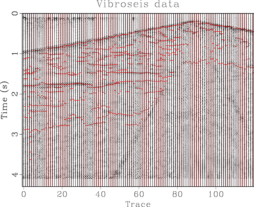
The second dataset is dataset 2 from Yilmaz (2001) and is shown in Figure 5. It is a 120-trace shot gather with 100 ft trace spacing and sampling interval 4ms. The source used to acquire this dataset is Vibroseis. Regarding this second dataset, we can make almost the same remarks as about the first one. Although the first breaks are identified, they are not accurately determined. As mentioned previously, first breaks can be identified accurately even in Vibroseis data (Saragiotis and Alkhalifah, 2012). However, other events are properly picked, including the reflections at about 1.5 and 1.8 s.
We reiterate that for both datasets, picking is performed without any preprocessing of the data and by applying the method to each trace separately, without taking into account information from neighboring traces. Such information is expected to enhance the picking performance significantly and is the subject of ongoing research.
Finally, the computational efficiency of the proposed method depends largely on the computational efficiency of the time-frequency transform and the operator that maps the time-frequency domain to the time domain. The algorithm by Liu et al. (2011) has the advantage of being easily parallelizable. Recently, efficient algorithms for computing time-frequency transforms, as for example in (Brown et al., 2010), have been introduced. Such efficient algorithms are expected to increase the computational efficiency of the proposed method.
|
|---|
|
oz6
Figure 4. oz6 |
|
|
|
|---|
|
oz2
Figure 5. Dataset 2 from (Yilmaz, 2001) and picked events (red). For displaying purposes, AGC has been applied on the data. |
|
|
|
|
|
|
Automatic traveltime picking using the instantaneous traveltime |