|
|
|
|
Velocity continuation by spectral methods |
The first problem is the loss of information in the transform to the
![]() grid. As illustrated in Figure 2, the shallow part of
the data gets severely compressed in the
grid. As illustrated in Figure 2, the shallow part of
the data gets severely compressed in the ![]() grid. The amount of
compression can lead to inadequate sampling, and as a result, aliasing
artifacts in the frequency domain. Moreover, it can be difficult to
recover from the loss of information in the transformed domain when
transforming back into the original grid. A partial remedy for this
problem is to increase the grid size in the
grid. The amount of
compression can lead to inadequate sampling, and as a result, aliasing
artifacts in the frequency domain. Moreover, it can be difficult to
recover from the loss of information in the transformed domain when
transforming back into the original grid. A partial remedy for this
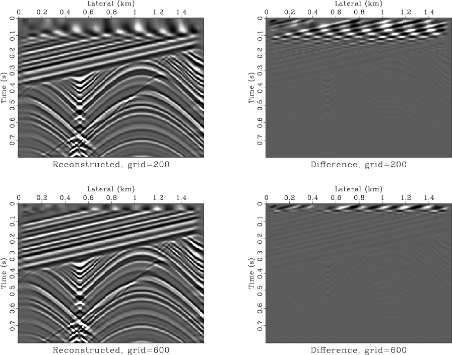
problem is to increase the grid size in the ![]() domain. The top plots
in Figure 4 show the result of back transformation to
the
domain. The top plots
in Figure 4 show the result of back transformation to
the ![]() grid and the difference between this result and the original
model (plotted on the same scale). We can see a noticeable loss of
information in the upper (shallow) part of the data, caused by
undersampling. The bottom plots in Figure 4 correspond
to increasing the grid size by a factor of three. Some of the
artifacts have been suppressed, at the expense of dealing with a
larger grid.
grid and the difference between this result and the original
model (plotted on the same scale). We can see a noticeable loss of
information in the upper (shallow) part of the data, caused by
undersampling. The bottom plots in Figure 4 correspond
to increasing the grid size by a factor of three. Some of the
artifacts have been suppressed, at the expense of dealing with a
larger grid.
|
|---|
|
fft-inv
Figure 4. The left plots show the reconstruction of the original data after transforming back from the |
|
|
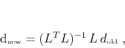
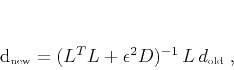
To perform an accurate transform of the grid, I adopted the following
method, inspired by (Claerbout, 1986a). Let
![]() denote the data on the new grid and
denote the data on the new grid and
![]() be the data on the old grid. If
be the data on the old grid. If ![]() is the interpolation operator,
defined on the new grid, then the optimal least-square transformation
is
is the interpolation operator,
defined on the new grid, then the optimal least-square transformation
is
|
|
|
|
Velocity continuation by spectral methods |