next up previous [pdf]

Next: Velocity picking and slicing Up: Fomel: Velocity continuation Previous: Fourier approach

Numerical velocity continuation in the prestack domain

To generalize the algorithm of the previous section to the prestack case, it is 
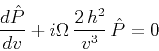
first necessary to include the residual NMO term (Fomel, 2003). Residual normal moveout can be formulated with the help of the differential equation:

\begin{displaymath}
{{\partial P} \over {\partial v}} +
{{h^2} \over {v^3 t}} {{\partial P} \over {\partial t}} = 0\;,
\end{displaymath} (10)

where $h$ stands for the half-offset. The analytical solution of equation (10) has the form of the residual NMO operator:
\begin{displaymath}
P(t,h,v) = P_0\left(\sqrt{t^2 + h^2 
\left(\frac{1}{v_0^2} - \frac{1}{v^2}\right)},h\right)\;.
\end{displaymath} (11)

After transforming to the squared time $\sigma = t^2$ and the corresponding Fourier frequency $\Omega$, equation (10) takes the form of the ordinary differential equation
\begin{displaymath}
\frac{d \hat{P}}{d v} +
i \Omega \frac{2 h^2}{v^3} \hat{P} = 0
\end{displaymath} (12)

with the analytical frequency-domain phase-shift solution
\begin{displaymath}
\hat{P} (\Omega, h, v) = \hat{P_0} (\Omega,h) e^{i \Omega h^2 
\left(\frac{1}{v_0^2} - \frac{1}{v^2}\right)}\;.
\end{displaymath} (13)

To obtain a Fourier-domain prestack velocity continuation algorithm, one just needs to combine the phase-shift operators in equations (9) and (13) and to include stacking across different offsets. The exact velocity continuation theory also includes the residual DMO term (Fomel, 2003), which has a second-order effect, pronounced only at small depths. It is neglected here for simplicity. The algorithm takes the following form:
  1. Input a set of common-offset images, migrated with velocity $v_0$.
  2. Transform the time axis $t$ to the squared time coordinate: $\sigma = t^2$.
  3. Apply a fast Fourier transform (FFT) on both the squared time and the midpoint axis. The squared time $\sigma $ transforms to the frequency $\Omega$, and the midpoint coordinate $x$ transforms to the wavenumber $k$.
  4. Apply a phase-shift operator to transform to different velocities $v$:
    \begin{displaymath}
\hat{P}(\Omega,k,v) = \sum_{h} \hat{P}_0 (\Omega,k,h) 
...
...mega h^2  \left(\frac{1}{v_0^2} -
\frac{1}{v^2}\right)}\;.
\end{displaymath} (14)

    To save memory, the continuation step is immediately followed by stacking. For velocity analysis purposes, a semblance measure (Neidell and Taner, 1971) is computed in addition to the simple stack analogously to the standard practice of stacking velocity analysis.

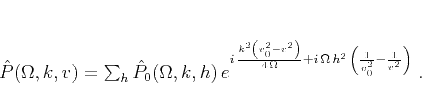
    Implementing the residual moveout correction in the Fourier domain allows one to package it conveniently with the phase-shift operator without the need to transform the continuation result back to the time domain. The offset dimension in equation (14) is replaced by the velocity dimension similarly to the velocity transform of the conventional stacking velocity analysis (Yilmaz, 2001).

  5. Apply an inverse FFT to transform from $\Omega$ and $k$ to $\sigma $ and $x$.
  6. Apply an inverse time stretch to transform from $\sigma $ to $t$.
One can design similar algorithms by using the finite difference method. Although the finite-difference approach offers a faster continuation speed, the spectral algorithm has a higher accuracy while maintaining an acceptable cost.

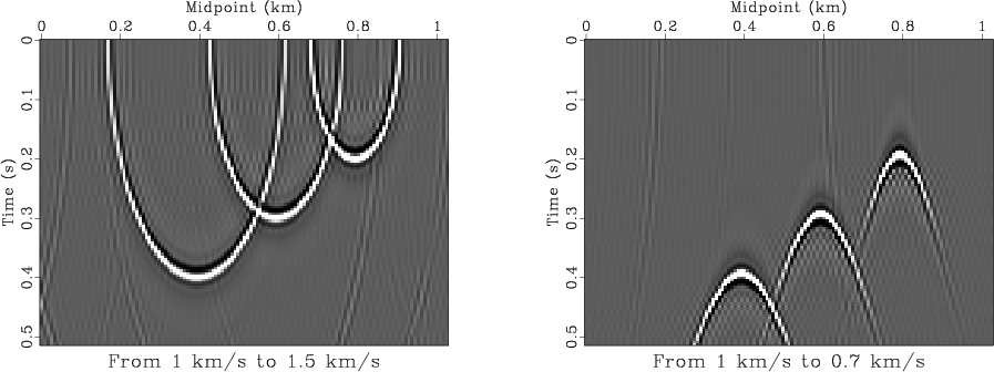
Figure 9 shows impulse responses of prestack velocity continuation. The input for producing this figure was a time-migrated constant-offset section, corresponding to an offset of 1 km and a constant migration velocity of 1 km/s. In full accordance with the theory (Fomel, 2003), three spikes in the input section transformed into shifted ellipsoids after continuation to a higher velocity and into shifted hyperbolas after continuation to a smaller velocity. Padding of the time axis helps to avoid the wrap-around artifacts of the Fourier method. Alternatively, one could use the artifact-free but more expensive Chebyshev spectral method (Fomel, 1998).

velimp
velimp
Figure 9.
Impulse responses of prestack velocity continuation. Left plot: continuation from 1 km/s to 1.5 km/s. Right plot: continuation from 1 km/s to 0.7 km/s. Both plots correspond to the offset of 1 km.
[pdf] [png] [scons]

Velocity continuation creates a time-midpoint-velocity cube (four-dimensional for 3-D data), which is convenient for picking imaging velocities in the same way as the result of common-midpoint or common-reflection-point velocity analysis. The important difference is that velocity continuation provides an optimal focusing of the reflection energy by properly taking into account both vertical and lateral movements of reflector images with changing migration velocity. An experimental evidence for this conclusion is provided in the examples section of this paper.

The next subsection discusses the velocity picking step in more detail.


Subsections
next up previous [pdf]

Next: Velocity picking and slicing Up: Fomel: Velocity continuation Previous: Fourier approach

2013-03-03