|
|
|
|
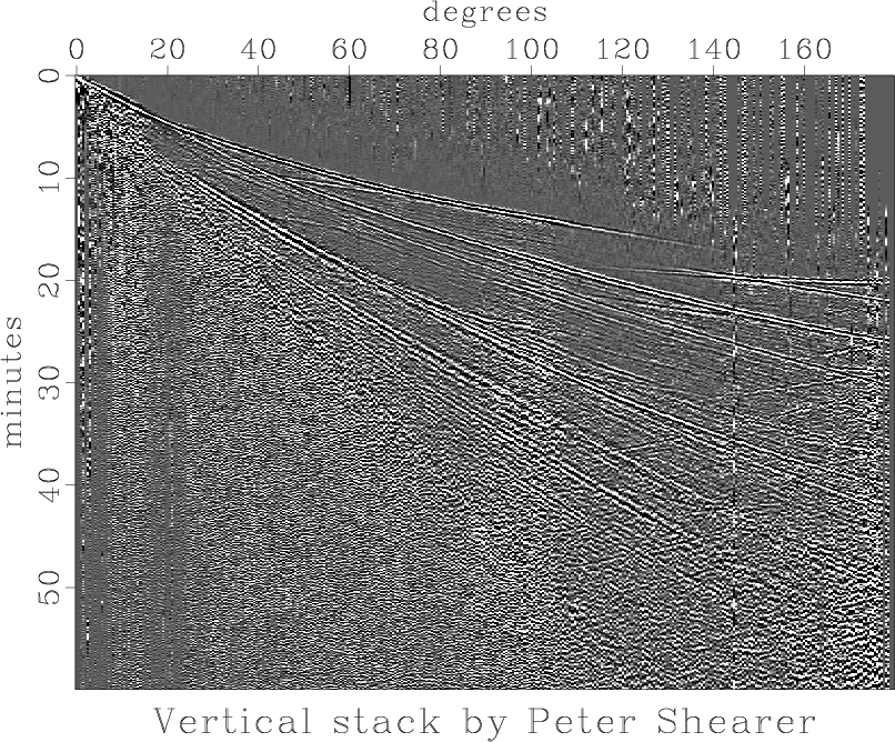
Earthquake stacks at constant offset |
Professor Shearer has found a way to choose the polarity for each seismogram so that the SH waves do not randomly cancel in the stack. Since SH waves have no conversions, the SH-wave stack in Figure 1 is easier to understand than the P-SV stack shown later. The first big event is direct S (shear wave). It comes tangent to ScS (reflection from the earth's core) hitting grazing angle around 90 degrees at about 23 minutes of travel time. The first multiple reflection of ScS at grazing angle is at double the epicentral distance and double the travel time. It is easily seen at the opposite side of the earth near 180 degrees offset. Figure 1 also shows six bounces of direct S bouncing from the earth's surface before the plot ends at one hour travel time. Incidentally, many fewer earthquakes are observed near 180 degrees than near 90 degrees for the simple geometrical reason that ten degrees surrounding the equator is a much bigger area than ten degrees surrounding the pole. Thus the quality of the stacks degrades rapidly toward the poles.

|
|---|
|
reftran
Figure 1. Transverse component. SH waves. |
|
|
Waves analogous to familiar water-bottom pegleg multiples are readily seen tracking S about 4 minutes later than S. The data shows these two events, one being a reflection from a layer at 410 km and the other from 660 km. As with familiar water-bottom peglegs, each event is a superposition of two events, one with a short path near the source and the other with a short path near the receiver.
Of particular interest are waves identified by Professor Shearer that track SS, the first surface multiple of S, but arrive about 4 minutes earlier. Were it not for the confusing similarity between ``shear'' and ``Shearer'', I would call these ``Shearer'' waves. They arrive earlier than the first multiple of direct S because instead of an earth-surface bounce at the middle of the path, they bounce a little sooner from the underside of the layers at 660 km and 410 km. The nice thing about Shearer's waves is that they are uniquely associated with the middle of the path, rather than having two bounce locations, as do familiar first-order peglegs. We might like to search our files of exploration data to see if we can find analogous events.
In the stack in Figure 2, Professor Shearer has chosen the polarities of each seismogram so that P-SV waves stack in phase. Because of conversions between P and SV, there are a huge number of new events which I leave to you to pick out. Waves that propagate further than 180 degrees fold back (like discrete Fourier transforms). I cannot explain why such folding was not visible on the SH section.
|
|---|
|
refvert
Figure 2. Vertical component showing P and SV waves. |
|
|
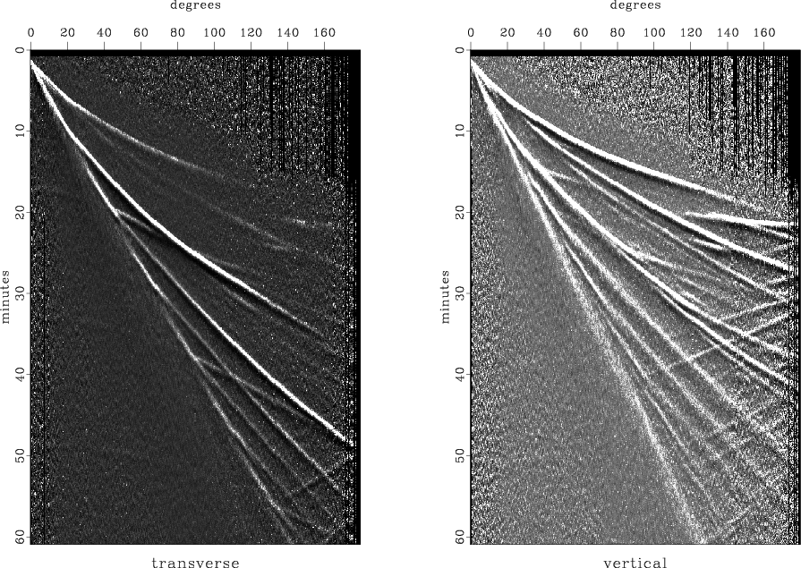
Figure 3 is a plot of signal amplitudes. These were the first stacks that Professor Shearer made because they require no knowledge of polarity.
|
|---|
|
anis
Figure 3. Transverse and vertical component of signal magnitude. See if you believe in whole-earth anisotropy. |
|
|
A challenging goal is to redo these stacks from the original data trying to boost the spectral bandwidth of the final result. This involves statics corrections and corrections for source depth.
|
|
|
|
Earthquake stacks at constant offset |