Multidimensional recursive filter preconditioning in geophysical estimation problems

Multidimensional recursive filter preconditioning

Claerbout (1998) proposed a helix transform for mapping multidimensional convolution operators to their one-dimensional equivalents. This transform proves the feasibility of multidimensional deconvolution, an issue that has been in question for more than 25 years (Claerbout, 1976). By mapping discrete convolution operators to one-dimensional space, the inverse filtering problem can be conveniently recast in terms of recursive filtering, a well-known part of the digital filtering theory.

helix
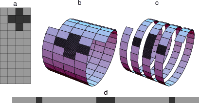
Figure 10. Helix transform of two-dimensional filters to one dimension (a scheme). The two-dimensional filter (plot a) is equivalent to the one-dimensional filter in (plot d), assuming that a shifted periodic condition is imposed on one of the axes (plots b and c.)

The helix filtering idea is schematically illustrated in Figure . The left plot (labeled ``a'' in the figure) shows a two-dimensional digital filter overlayed on the computational grid. A two-dimensional convolution computes its output by sliding the filter over the plane. If we impose helical boundary conditions on one of the axes, the filter will slide to the beginning of the next trace after reaching the end of the previous one (plot ``b''). As evident from plots ``c'' and ``d'', this is completely equivalent to one-dimensional convolution with a long 1-D filter with internal gaps. For efficiency, the gaps are simply skipped in a helical convolution algorithm. The gain is not in the convolution itself, but in the ability to perform recursive inverse filtering (deconvolution) in multiple dimensions. A multi-dimensional filter is mapped to its 1-D analog by imposing helical boundary conditions on the appropriate axes. After that, inverse filtering is applied recursively in a one-dimensional manner. Neglecting parallelization and indexing issues, the cost of inverse filtering is equivalent to the cost of convolution. It is proportional to the data size and to the number of non-zero filter coefficients.

waves
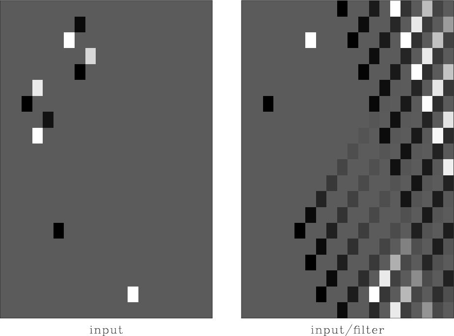
Figure 11. Illustration of 2-D deconvolution with helix transform. Left is the input: two spikes and two filters. Right is the output of deconvolution.

An example of two-dimensional recursive filtering is shown in Figure 11. The left plot contains two spikes and two filter impulse responses with different polarity. After deconvolution with the given filter, the filter responses turn into spikes, and the initial spikes turn into long-tailed inverse impulse responses (right plot in Figure 11). Helical wrap-around, visible on the top and bottom boundaries, indicates the direction of the helix. Claerbout (1999) presents more examples and discusses all the issues of multidimensional helical deconvolution in detail.

Multidimensional recursive filter preconditioning in geophysical estimation problems